← writing, Science Olympiad, hardware, Oct 16, 2026
Building a water salinity detector for Science Olympiad
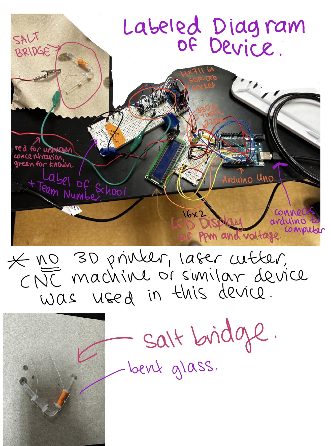
For Science Olympiad Detector Building, the event hands you a measurable quantity and asks you to build something that reads it. The year my partner Nathan Chiu and I competed, the quantity was water salinity, the concentration of dissolved salt in a sample. We had to design a device that took in an unknown water sample and reported its salinity, built from parts we could wire ourselves. The rules banned 3D printers, laser cutters, and CNC machines, so everything sat on a wooden board we held together with epoxy.
We competed under Bothell High School and built the device across the 2022 to 2024 seasons. We placed 1st at every regional and state competition we entered, and we won the MIT national invitational in 2024.
How it reads salt from a voltage
The core of the device is a salt bridge. I bent a piece of glass tubing into a U, filled it with agar that held dissolved potassium chloride, and set each end into a different cup of water. One cup holds a reference solution whose salinity I already know. The other holds the unknown sample. The salt bridge lets ions move between the two solutions without letting the liquids mix, which closes an electrical circuit between them.
Two solutions of different salt concentration, connected this way, behave like a weak battery, a concentration cell. The bigger the difference in concentration, the larger the voltage that builds across the bridge. That voltage is what we measure. The Nernst equation ties the two together, and it says the cell voltage grows with the logarithm of the ratio of the two concentrations. A small voltage near zero means the sample sits close to the reference, and a growing voltage means it sits far from it.
A wire runs from each end of the salt bridge to the electronics. From there the device reads a very small voltage and turns it into a salinity number on a screen.
The electronics
An Arduino Uno runs the device. It cannot read microvolt-level signals on its own, so the voltage across the salt bridge passes through an HX711, a 24-bit analog-to-digital converter that amplifies tiny voltages before the Arduino sees them. The HX711 reads signals down in the microvolt range, the scale a concentration cell produces. We seated the HX711 chip in a SOP-16-to-DIP-16 socket so it would sit on a breadboard, and the chip carries its own resistors and capacitors.
The Arduino drives a 16x2 LCD that prints the measured voltage on the top line and the salinity in parts per million on the bottom line. Three resistor-LED pairs give a quick color readout of which concentration band the sample falls into. We also ran a red lead and a green lead for the two cups, red for the unknown sample and green for the reference.
Here is the main loop of the Arduino sketch. It averages ten readings from the HX711, holds the value steady when it drifts by less than half a percent to stop slow creep, converts the raw count to microvolts, and lights the LED for whichever band the reading falls in.
#include "HX711.h"
#include "LiquidCrystal.h"

#define BLUE 10
#define GREEN 9
#define RED 8

LiquidCrystal lcd(12, 11, 5, 4, 3, 2);
const int DOUT1 = 6; const int SCK1 = 7; HX711 scale;

// concentration bands, in ppm, for the three indicator LEDs
const double b1 = 0.0;    const double b2 = 2000.0; // blue
const double g1 = 2000.0; const double g2 = 4000.0; // green
const double r1 = 4000.0; const double r2 = 5000.0; // red

void loop() {
  static long total = 0;
  static int times = 0;
  static double prevV = 0.0;

  double voltage = scale.get_value(10);              // average of 10 raw reads
  if (abs(voltage - prevV) < voltage / 200) voltage = prevV; // hold if < 0.5% change
  prevV = voltage;

  if (voltage > 50) {
    int v = scale.get_value(10);
    total += v / 4.5;                                // raw count to microvolts
    times += 1;
    long ppm = round(total / times * 1.0);

    lcd.setCursor(0, 0); lcd.print("Voltage:"); lcd.print(round(total / times)); lcd.print("uV");
    lcd.setCursor(0, 1); lcd.print("p:"); lcd.print(ppm); lcd.print("ppm");

    digitalWrite(BLUE,  (b1 < ppm && ppm < b2));
    digitalWrite(GREEN, (g1 < ppm && ppm < g2));
    digitalWrite(RED,   (r1 < ppm && ppm < r2));
  }
}
Calibration
The wiring was quick. Most of the season went into turning the voltage readings into salinity numbers. A raw voltage means nothing until you know what concentration produced it, so we mixed samples at concentrations we knew, read the voltage for each one, and recorded the pairs. That table is the calibration.
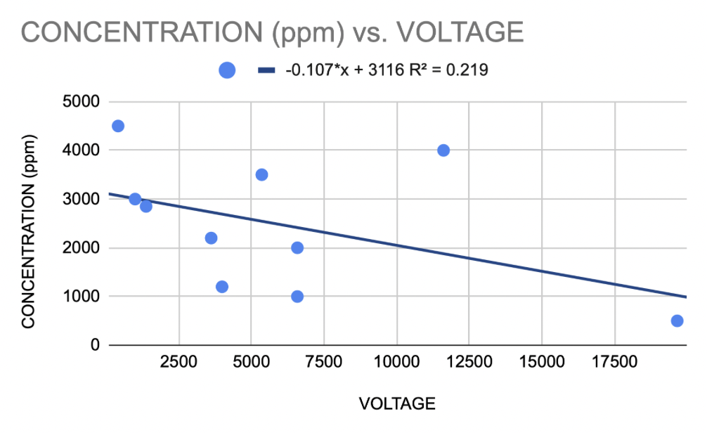
Our early attempts were rough. On one of the first full calibration runs, ten samples gave a scatter that barely trended at all, and the line of best fit explained only about a fifth of the variation (R-squared near 0.22). The points sat in almost a cloud, which told us the device was picking up as much noise as signal.
Two changes fixed it. The HX711 averaging and the creep filter cut the jitter in each reading. Then I treated the sensor as a logarithmic device from the start, since the Nernst relationship is logarithmic, and fit concentration against the log of the voltage instead of the voltage itself. An earlier version of our code used a log fit directly, computing concentration roughly as a constant minus 633 times the natural log of the reading, with the exact coefficients shifting between versions.
By the end, a clean calibration sweep looked like this, with voltage in microvolts against the known concentration in ppm:
| Voltage (uV) | Concentration (ppm) |
|---|---|
| 0 | 0 |
| 252 | 147 |
| 544 | 297 |
| 893 | 504 |
| 1210 | 654 |
| 1580 | 854 |
| 1770 | 954 |
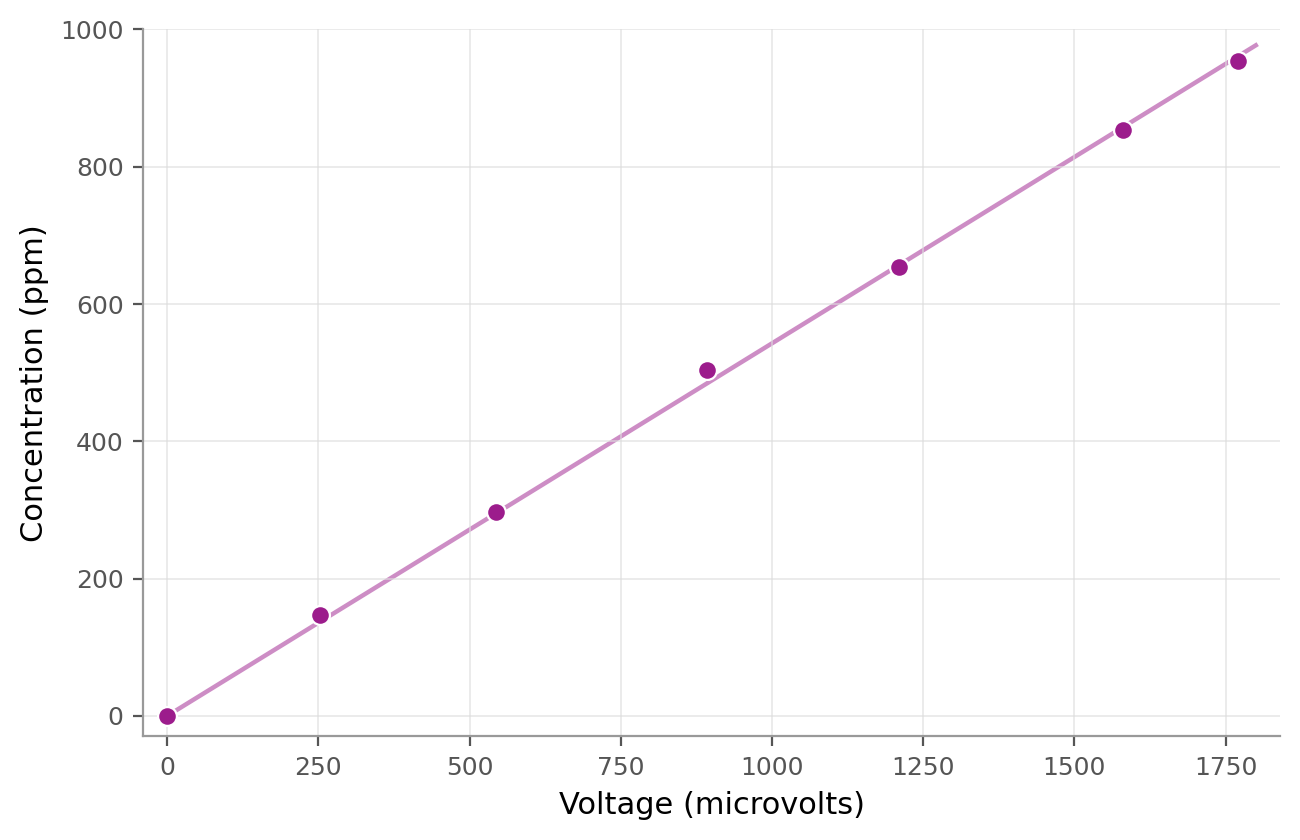
Across the full sweep the relationship held close to a straight line through the origin. 1770 microvolts mapped to about 954 ppm, a little more than half a ppm for every microvolt, and the intermediate points sat near that same slope. Turning that cloud of points into a line I could trust is the part of the project I am most proud of.
What I learned
Building the sensor was the quick part. The salt bridge and the electronics worked once I understood what each piece did. The measurement took much longer. I spent far more hours mixing known samples and plotting voltage against concentration than I spent soldering.
The calibration also taught me to check the chemistry when the numbers looked off. Our first scatterplots had no clear trend, and the reason was that a concentration cell follows a log curve, so a straight-line fit could not work. Fitting against the log of the voltage fixed it. Now I check what shape the physics predicts before I fit a model to anything.