Reading the brain, a guide to neural interfaces and clinical decoding

TL;DR. A brain-computer interface (BCI) reads signals from the nervous system, writes signals into it, or both, to restore or extend what a person can do. Over the last two decades the field has gone from monkeys moving cursors to people with paralysis typing with both hands, speaking through a decoder at speeds approaching conversation, feeling touch through a robotic hand, and seeing patterns drawn directly onto visual cortex. This guide works through roughly thirty-one papers, most of them primary studies, and reads each one alongside the mathematics and physics that make it possible. I begin with how the cortex is organized, develop population coding and the decoders that turned recorded spikes into movement, and then move through cognitive signals in parietal cortex, recording modalities, representational stability, latent dynamics, microstimulation for touch, prostheses for sight and hearing, speech and inner-speech decoding, closed-loop neuromodulation for depression, and functional ultrasound. In each section I pair a close reading of the papers with derivations and simulations that show why the methods work and where they fail. Every simulated number comes from the companion code, and every number attributed to a paper comes from that paper.

This guide grew out of a course on brain-computer interfaces that Professor Richard Andersen taught at Caltech, in which each week paired two primary papers with a guest lecture. The reading list spanned almost a century, from Wilder Penfield’s 1937 stimulation maps to a 2026 study in which two people with paralysis typed with both hands through an implanted neuroprosthesis. Read in order, the papers tell a coherent story, and my aim here is to make the connections between them explicit. BCIs sit at the intersection of neuroscience, electrical engineering, signal processing, machine learning, clinical medicine, and ethics, and each paper assumes a reader who already knows the ideas from the field next door. A paper on speech decoding assumes you know what threshold crossings are, why recurrent networks are trained with connectionist temporal classification, and why the same decoder, with a phoneme error rate near 20%, produced a word error rate of 9.1% under a 50-word language model and 23.8% with a 125,000-word vocabulary. A paper on tactile feedback assumes you know why charge density limits stimulation amplitude and what a projected field is. A paper on decoder stability assumes familiarity with factor analysis and Procrustes alignment. Textbooks in different fields cover these ideas separately, so I gather them here at the depth needed to read the primary literature critically.

The guide runs in fourteen sections. The first four build up the neuroscience, covering how the cortex is laid out, how populations of neurons encode variables, how recorded spikes become movement, and what cognitive signals posterior parietal cortex adds. The next three concern the engineering of reading, namely which sensor to use, whether neural representations stay put, and how latent dynamical models recover single-trial structure. The next three turn to writing and to sensory restoration, covering microstimulation for touch, prostheses for sight and hearing, and speech and typing neuroprostheses. The last four treat harder frontiers, namely inner speech and mental privacy, closed-loop neuromodulation for depression, functional ultrasound as a less invasive window, and the open problems the whole reading list leaves behind. Within each section I first build the background, then read each paper closely, with a shaded summary of its question, approach, and finding, and then connect the papers to each other. I derive a method wherever it is central, and a companion simulation shows each method recovering a known ground truth, and where it breaks down. The notation is standard. Vectors sit in bold lowercase (\(\bm{x}\)), matrices in bold uppercase (\(\bm{A}\)), neural activity at time \(t\) is written \(\bm{z}_{t} \in \mathbb{R}^N\) for \(N\) channels, decoded behavior \(\bm{x}_{t}\), and \(\mathcal{N}(\bm{\mu}, \bm{\Sigma})\) a Gaussian.

Before turning to the papers, I want to lay out in my own terms the measurement trade that sits underneath all of them. The rest of this guide reads the literature against the frame built in these three short sections, and I return to my own clinical work with it later on.

The three axes

Three mostly independent properties determine how useful a neural interface is. Spatial resolution is how small a region it can distinguish, from whole lobes down to single neurons. Temporal resolution is how fast a change it can follow, from seconds down to milliseconds. Invasiveness is how much of the skull and brain you have to open, from a cap on the scalp to electrodes in the tissue. Where a method lands on all three at once sets its usefulness for a given question, and almost nothing lands well on all three.

The physics forces the trade. The skull and scalp smear the electrical signals measured at the scalp, so EEG reads fast and localizes only coarsely. The blood-oxygen signal fMRI measures is sharp in space and lags neural activity by seconds, so it reads where with timing that trails the activity. To get both at once you put the sensor next to the neurons, which means surgery.

showing: all methods bottom-left is best on both axes; color marks invasiveness

Take the methods one by one. Scalp EEG records electrical potentials from a cap of electrodes. Timing is excellent, on the order of a millisecond, and it is cheap and fully non-invasive, which is why it dominates clinical epilepsy and brain-computer interfaces. Its spatial resolution is poor, on the order of centimeters, because every electrode sums the activity of enormous populations seen through the skull. MEG reads the magnetic fields of the same currents. Its timing matches EEG and its spatial resolution is somewhat better because magnetic fields are less distorted by tissue, but it needs a shielded room and a large machine.

fMRI infers activity from blood oxygenation. Its spatial resolution reaches about a millimeter, good enough to separate small structures, but the blood response is slow, so its temporal resolution is on the order of a second. fNIRS uses light to read a similar blood signal and is portable, at worse resolution on both axes.

ECoG places an electrode grid directly on the cortical surface, under the skull. It recovers millimeter space and millisecond time at once, the combination that stays out of reach from outside the skull, at the cost of surgery. Intracortical arrays, the Utah array and the penetrating threads used by implant companies, push further, resolving individual neurons with millisecond timing, at the cost of putting electrodes into the tissue itself. These are the recordings behind the most capable motor and speech decoders, and surgery is the price of that access.

This matters for machine learning because a decoder recovers only information the sensor captured. A model reading scalp EEG inherits EEG’s spatial blur no matter how good the model is, so asking it to name the exact region a signal came from asks it to invert a measurement that already threw that information away. I have run into this directly in epilepsy work. Localizing a lesion from EEG is hard because the modality safe enough to use routinely is the one with the least spatial information. The modality sets the main limit here. In my own analysis, most of the apparent spatial performance of an EEG localizer was label frequency, and the spatial signal localized only about 1.6 times over its own blind floor. That is a statement about the modality as much as the model.

This is also why the implant companies accept surgery. If you need single-neuron resolution and millisecond timing, surgery is the only way to get them, and the entire value of a penetrating electrode is that it buys the good corner of the trade that physics closes off from the outside. The right interface is the one whose fixed point on the three axes matches the question, and whose invasiveness the application can justify.

The cortex as a map

Every BCI starts with a decision about where to put the sensor. A surgeon implanting a microelectrode array chooses a patch of cortex a few millimeters across, and that choice fixes what the device can read. If the patch represents the hand, a decoder can recover attempted hand movements; if it represents the face, the same decoder will find little to work with. Surgeons base the decision on a picture of the cortex as a map, in which each body part has its own territory and neighbors occupy neighboring territories. That picture is almost a century old, and in several important ways it is wrong.

Motor and somatosensory cortex lie on either side of the central sulcus, motor in front and somatosensory behind, each strip running roughly from leg near the midline to face near the side of the head. On structural MRI the precentral gyrus bends into a shape like an inverted omega at the hand representation, the “hand knob,” and its reliability is the main reason many intracortical BCIs, including the BrainGate trials, place arrays there. Three methods ask “where” in different ways and at different scales. Direct electrical stimulation tests sufficiency, since a positive response shows that activating tissue near the electrode is enough to produce an effect. Functional MRI (fMRI) measures the blood-oxygenation (BOLD) signal, which is correlational, covers the whole brain, and unfolds over seconds. Single-unit and multi-unit recording resolve individual neurons or small groups at millisecond scale but sample only a few square millimeters. Each answers a different question, so maps made with different methods can disagree.

We can make the idea of a map precise. Let \(\bm{s} \in B \subset \mathbb{R}^2\) be a point on the flattened skin and \(\bm{c} \in C \subset \mathbb{R}^2\) a point on the flattened cortex. A somatotopic map is a function \(\bm{c} = \bm{\phi}(\bm{s})\) that assigns each skin location the cortical location representing it. If \(\bm{\phi}\) is differentiable, a small skin patch spanned by \((\delta s_{1}, 0)\) and \((0, \delta s_{2})\) maps to a parallelogram whose area is the absolute determinant of the Jacobian \(\bm{J} = \partial \bm{\phi}/\partial \bm{s}\) times the patch area, so the cortical territory of a body part \(P\) is

\[A_{C}(P) = \int_{P} \vert \det \bm{J}(\bm{s})\vert \, dA_{B} .\]

We call \(M(\bm{s}) = \vert \det \bm{J}(\bm{s})\vert\) the areal magnification. A large territory can come from a large body part or from high magnification; the hand is small, so its large territory means its magnification is high. The homunculus is a picture of this magnification. One common hypothesis is that each unit of cortex processes a roughly fixed number of peripheral fibers, so \(M(\bm{s}) \propto \rho(\bm{s})\) for fiber density \(\rho\), which is why densely innervated skin such as fingertips and lips receives more cortex. The formal picture assumes continuity, a single body location per cortical point, and that the map is the only organization of the sheet. Cortex itself violates all three.

Penfield and Boldrey (1937) stimulated the exposed cortex of 126 awake patients under local anesthesia, recorded which body part moved or tingled, and condensed the results into the first homunculus. (The full text was unavailable to me, so this account rests on secondary sources, chiefly Catani’s 2017 reanalysis.) Body parts followed an orderly sequence from leg near the midline to face and tongue laterally, but with substantial overlap, and motor and sensory responses appeared on both sides of the central sulcus. Edwin Boldrey sketched 170 summary maps from Penfield’s notes, pooling points from different patients onto one template by eye, with no statistics, and the drawing sized each body part by the vertical extent of its representation, a one-dimensional magnification in place of an areal one. Gordon and colleagues, citing Penfield, note that stimulation elicited movement from only about half of sites, and that earlier accounts left the sites producing no movement undocumented. Pooling can make a sequence look clean even when a single patient shows only part of it, and turning overlapping maps into one drawing discards which body parts share cortex. Penfield himself, in his 1950 monograph, called the drawing “an aid to memory.”

Mountcastle’s 1997 review restated his columnar hypothesis, that cortical areas consist of local circuits repeated many times, a column being many minicolumns bound by short-range horizontal connections, with links among modules in different areas forming nested distributed systems. (I had only the abstract and secondary sources.) Later reviewers objected that the number of minicolumns making a column remains unspecified, and that no repeating canonical circuit maps one-to-one onto the minicolumn; Horton and Adams called the column “a structure without a function.” The modular view arose in sensory cortex, where peripheral submodalities could define columns, and its extension to motor and association cortex, the areas BCIs care about, has less support. One practical point holds regardless. A Utah array spans an area many times wider than a putative column, so what its electrodes carry together reflects a population drawn from many units. That is one reason population coding is the basic language of BCIs.

Willett and colleagues (2020) measured the hand-knob map at single-neuron resolution. Recording multi-unit activity from two Utah arrays in each of two BrainGate2 participants with tetraplegia, they found that all tested movements of the face, head, arms, and legs modulated hand-knob activity, with tuning heavily intermixed and no clear somatotopy. In this paper, a patch surgeons pick for its hand representation carried tuning to the face and legs. As a fraction of arm tuning (the strongest), face tuning was 38% in both participants, head tuning 46% and 34%, and leg tuning 61% and 53%. The code for limbs was compositional. If the population response to “move limb \(\ell\) in manner \(m\)” is \(\bm{x}_{\ell m} = \bm{\mu} + \bm{a}_\ell + \alpha\,\bm{v}_{m} + \beta\,\bm{w}_{\ell m}\), with \(\bm{a}_\ell\) coding the effector, \(\bm{v}_{m}\) a shared movement component, and \(\bm{w}_{\ell m}\) an effector-specific interaction, then after subtracting the mean within each laterality the correlation between the same movement on two limbs is

\[r_{\text{match}} = \frac{\alpha^2\|\tilde{\bm{v}}_{m}\|^2}{\alpha^2\|\tilde{\bm{v}}_{m}\|^2 + \beta^2\|\tilde{\bm{w}}\|^2},\]

the fraction of pattern energy carried by the shared component. Matching arm movements had mean \(r = 0.52\) against \(-0.07\) for non-matching pairs; for the leg, \(0.73\) against \(-0.14\); and homologous arm-and-leg movements such as a hand grasp and a toe curl also correlated. Matching correlations stayed between about 0.5 and 0.7, so the code is partially compositional. A whole-body discrete BCI drawing targets from four limbs achieved a higher bit rate than one using a single wrist, because spreading targets across limbs that occupy partly different neural dimensions avoids crowding the nearest-neighbor distances that govern errors. Two simulated recurrent networks, one with compositional inputs and one with a direct input per arm, both produced 100% of units tuned to both arms, so intermixed single-unit tuning is compatible with different population codes. Mixing is a property of the population.

Gordon and colleagues (2023) used hours of fMRI per person to show that primary motor cortex contains structure beyond the effector map. Reliable resting-state connectivity needs a great deal of data in one person, because the BOLD time series is strongly autocorrelated. For a first-order autoregressive process with coefficient \(\phi\), the effective sample size is \(n_{\text{eff}} = T\,(1-\phi^2)/(1+\phi^2)\) for the autocorrelation of a product; with \(\phi = 0.8\) this is about \(0.22\,T\), which is why precision functional mapping scans each person for hours. Averaging across people also blurs fine features, because a feature of width \(w\) whose center varies across people with standard deviation \(\sigma\) becomes a group feature of width \(\sqrt{w^2 + \sigma^2}\) with its peak lowered by \(w/\sqrt{w^2+\sigma^2}\). In seven highly sampled adults, Gordon and colleagues found that the foot, hand, and mouth regions of the precentral gyrus alternate with three “inter-effector” regions that connect strongly to each other and preferentially to the cingulo-opercular network and to subcortical and medial structures. They named the combined system the somato-cognitive action network (SCAN), proposed an “integrate-isolate” model in which effector regions isolate fine control while the SCAN integrates whole-body action planning and physiological control, and found that published motor stimulation sites fell outside the middle inter-effector region, offering one explanation for Penfield’s silent sites.

A few more of Willett’s results sharpen the picture. Ipsilateral movements also modulated the hand knob, with firing-rate changes 65% of contralateral for the arm and 78% for the leg, and a naive Bayes classifier told the full set of ipsilateral and contralateral movements apart at 97.4%. The compositional components prepared separately. When the cue named only the movement, the movement dimension partially prepared during the delay while the laterality dimension stayed put, and when the cue named only laterality the reverse happened, which argues that the decomposition reflects the brain’s own signals. The additive model breaks when two effectors move at once, since the secondary effector’s modulation weakens and its neural axis rotates, with the alignment between the two effectors’ axes falling from 0.33 to 0.14. This simultaneous-movement result constrains any BCI that decodes several effectors together, and it foreshadows the bimanual typing work later in this guide. In the terms of mixed selectivity, an additive limb-plus-movement code resembles linear mixed selectivity at the population level, and the departures during dual movement are a nonlinear interaction.

Gordon’s structural and developmental evidence rounds out the SCAN account. In all seven adults the inter-effector regions were more strongly connected to the cingulo-opercular network than the foot, hand, or mouth regions were, and inter-effector cortex was thinner, had higher fractional anisotropy beneath it, and carried myelin levels between those of the foot and hand regions. Task fMRI in two participants found that distal body parts sit at the center of each effector zone and proximal parts at the periphery, so the effector map folds back on itself along the strip, which in the formal language means the map is many-to-one. The motif was absent in neonates, detectable at 11 months, and almost adult-like at 9 years, and a dorsal anterior cingulate seed in a macaque connected to two candidate homologues of the inter-effector regions. Depth-electrode recordings have since found that the superior inter-effector region responds to foot, hand, and mouth movements, an early step toward testing the SCAN with direct neural recordings. Mountcastle’s claim that one cytoarchitectural area may belong to several distributed systems describes Gordon’s interleaved regions well, though his strong modular view fits Willett’s intermixed tuning poorly, since an array spanning many putative columns showed no patchy somatotopy.

Reading the four papers in sequence, they line up cleanly. The four papers show the same cortex at four scales. Penfield pooled surface stimulation across patients and scaled by linear extent; Gordon mapped individuals and found a region stimulation leaves silent; Willett recorded neurons and found that macroscopic order hides mixing within a single array. The most interesting open question is the relation between Willett and Gordon. Gordon suggests Willett’s whole-body tuning, recorded near the superior SCAN node, may reflect inter-effector activity, while Willett found the strongest tuning to the arm and a structured compositional code, which fits a hand-and-arm region better than a region with weak movement specificity. Deciding requires knowing where each array sat relative to the participant’s own SCAN map, which remains unestablished.

Population codes and mixed selectivity

Every intracortical BCI rests on a claim about how neurons carry information, that each neuron’s firing rate depends regularly on a behavioral variable, and that the regularity is shared widely enough that a few dozen or a few hundred neurons, sampled almost at random, suffice to recover the intended movement. This section asks where that claim came from and how far it extends beyond simple reaching.

A tuning curve \(f(\theta)\) gives a neuron’s mean firing rate as a function of a variable. In motor cortex, a neuron’s rate during reaching varies smoothly with direction, peaking in one preferred direction. We call a neuron cosine-tuned if \(f(\theta) = b_{0} + g\cos(\theta - \theta_{\mathrm{pref}})\), with baseline \(b_{0}\), gain \(g\), and preferred direction \(\theta_{\mathrm{pref}}\). This shape follows from a linear encoding model. If the rate depends linearly on velocity \(\bm{v} = s(\cos\theta, \sin\theta)^\top\), then \(f_{i} = b_{0,i} + s\|\bm{h}_{i}\|\cos(\theta - \theta_{i})\), so a linear model of a two-dimensional velocity produces only a cosine, and the preferred direction is the direction of the weight vector. A tuning curve narrower than a cosine, or with two peaks, is evidence of nonlinearity. This is why linear decoders work as well as they do in motor cortex.

Georgopoulos and colleagues (1986) proposed reading movement direction from the whole population. Let \(\bm{u}_{i}\) be neuron \(i\)’s preferred-direction unit vector and \(w_{i} = (r_{i} - b_{0})/g\) its baseline-subtracted weighted rate. The population vector is \(\bm{P} = \sum_{i} w_{i} \bm{u}_{i}\), and the decoded direction is its angle. Taking expectations, \(\mathbb{E}[\bm{P}] = \sum_{i} \cos(\theta-\theta_{i})\bm{u}_{i}\), and when preferred directions are spaced evenly the cross terms form a geometric series that sums to zero for \(N \ge 3\), leaving \(\mathbb{E}[\bm{P}] = (N/2)(\cos\theta,\sin\theta)^\top\) pointing in the true direction. The matrix form makes the fix for non-uniform directions clear. Writing \(\mathbb{E}[\bm{P}] = \bm{M}\,\bm{u}(\theta)\) with \(\bm{M} = \sum_{i} \bm{u}_{i}\bm{u}_{i}^\top\), the estimate is unbiased if and only if \(\bm{M}\) is proportional to the identity. With independent Poisson noise the variance of the angle falls as

\[\mathrm{Var}(\delta) \approx \frac{2 b_{0}}{N T g^2},\]

so error falls as \(1/\sqrt{N}\), and doubling the window has the same effect as doubling the neurons. Fisher information gives a lower bound with the same scaling. For cosine tuning \(J \approx NT(b_{0} - \sqrt{b_{0}^2 - g^2})\), and with the companion parameters (\(b_{0} = 10\) Hz, \(g = 8\) Hz, \(T = 0.2\) s) the Cramér-Rao bound on the standard deviation is \(1.118/\sqrt{N}\) radians, while the population vector reaches \(1.25/\sqrt{N}\), about 12% above the bound. I ran this simulation myself, and a decoder this simple lands only 12% above the information-theoretic floor. The optimal linear estimator removes the population vector’s bias by multiplying it by a correction matrix that approaches \(\bm{M}^{-1}\) in the low-noise limit.

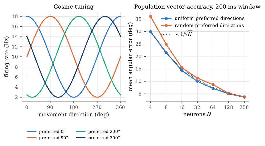
Figure 1. Cosine tuning and population-vector accuracy. Left, tuning curves \(f(\theta) = 10 + 8\cos(\theta - \theta_{\mathrm{pref}})\) Hz for four neurons with preferred directions of 0, 90, 200, and 300 degrees. Right, the mean absolute angular error of the population vector against the number of Poisson neurons \(N\), decoded from spike counts in a 200 ms window and averaged over 2000 random directions. With uniformly spaced preferred directions the error falls from 29.95 degrees at \(N=4\) to 3.60 degrees at \(N=256\); randomly drawn directions give slightly higher errors because the cross terms no longer cancel. The dotted line is a \(1/\sqrt{N}\) reference. Simulated data from the companion code.

Most of cortex encodes several variables at once. For two binary variables \(a\) and \(b\), recoded as \(s_{a}, s_{b} \in \{-1, +1\}\), any neuron’s mean response is \(r_{i} = \mu_{i} + \alpha_{i} s_{a} + \beta_{i} s_{b} + \gamma_{i} s_{a} s_{b}\), a two-way ANOVA. A neuron is purely selective if only one main effect is nonzero, linearly mixed if both main effects are nonzero but \(\gamma_{i} = 0\), and nonlinearly mixed if \(\gamma_{i} \ne 0\). The review by Tye and colleagues (2024) develops the geometric consequence. Collecting the centered condition means into \(\bm{R}_{c} = \bm{s}_{a}\bm{\alpha}^\top + \bm{s}_{b}\bm{\beta}^\top + \bm{s}_{ab}\bm{\gamma}^\top\), its rank is at most 3; if every neuron is pure or linearly mixed (\(\bm{\gamma} = \bm{0}\)) the rank is at most 2, however many neurons there are. Only nonlinear mixing lifts the condition means out of a plane. This matters because a linear readout computes \(y = w_{0} + \bm{w}^\top\bm{r} = c_{0} + (\bm{w}^\top\bm{\alpha})s_{a} + (\bm{w}^\top\bm{\beta})s_{b} + (\bm{w}^\top\bm{\gamma})s_{a}s_{b}\), and exclusive-or (XOR) requires the \(s_{a}s_{b}\) term. If \(\bm{\gamma} = \bm{0}\), adding the correct-at-corners inequalities forces both \(c_{0} < 0\) and \(c_{0} > 0\), a contradiction, so no linear readout separates XOR; if \(\bm{\gamma}\) has a component orthogonal to \(\bm{\alpha}\) and \(\bm{\beta}\), choosing \(\bm{w}\) along it gives \(y = -s_{a} s_{b}\), which separates it. A conjunctive neuron acts as a hidden layer that has already done the nonlinear work. Cover’s counting theorem makes the scaling precise. A linear threshold unit realizes \(C(P,d) = 2\sum_{k=0}^d \binom{P-1}{k}\) dichotomies of \(P\) points in general position in \(d\) dimensions. For four conditions in a plane, \(C(4,2) = 14\) of the 16 dichotomies, the two missing ones being XOR and its complement; in three dimensions, \(C(4,3) = 16\), all of them. High dimensionality has a cost, since a readout that can separate any dichotomy generalizes poorly, and fully mixing \(V\) variables needs on the order of \(2^V\) neurons; if two tasks each use a disjoint half of the variables, mixing within each needs only about \(2^{V/2+1}\), which for twenty variables is the difference between a million neurons and two thousand. This is why Tye and colleagues argue the brain should mix selectively, combining the variables a task needs and keeping others apart, gated by connectivity and perhaps by oscillations and neuromodulation. Rank is a fragile measure of dimensionality, since any noise makes a matrix full rank, so we use the participation ratio \(\mathrm{PR} = (\sum_{k}\lambda_{k})^2/\sum_{k}\lambda_{k}^2\), which equals the number of equal nonzero eigenvalues and gives an effective, variance-weighted count between those extremes. For two variables with orthogonal coefficient vectors of lengths 1, 1, and \(\varepsilon\), the participation ratio is \((2 + \varepsilon^2)^2/(2 + \varepsilon^4)\), which is 2 for a pure or linear mixed code and 3 when the interaction is as strong as the main effects, so it tracks how much of a third dimension actually exists, which is closer to what a noisy readout can use than rank is.

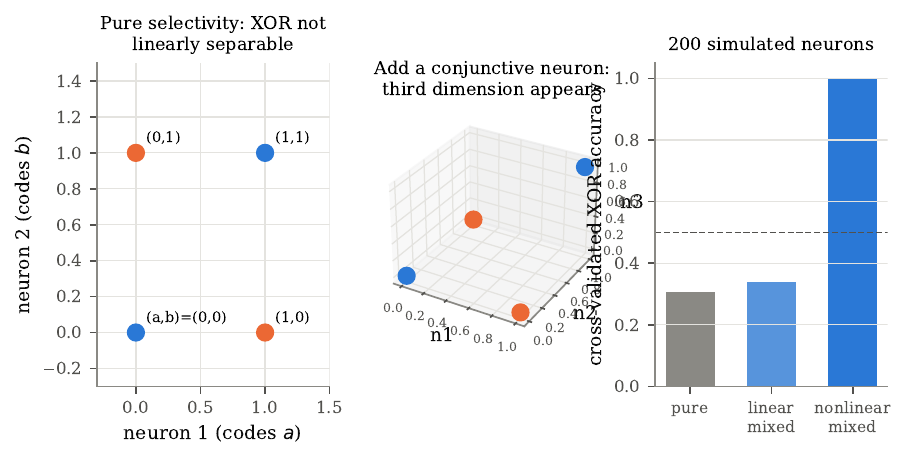
Figure 2. Mixed selectivity and linear decodability of exclusive-or. Left, two purely selective neurons place the four conditions at the corners of a square, and no line separates the two XOR labels. Middle, adding a conjunctive neuron whose rate is \(ab\) lifts one condition into a third dimension, after which a plane separates the labels. Right, cross-validated XOR accuracy of a linear classifier reading 200 simulated neurons: pure population 0.31, linear mixed 0.34, nonlinear mixed 1.00, with chance at 0.5. The rank of the centered condition means is 2, 2, and 3. The below-chance values for the pure and linear mixed populations are an artifact of cross-validating a labeling the classifier cannot learn, and should be read as chance. Simulated data from the companion code.

Two further tools help read the mixed-selectivity work. Demixed principal component analysis separates the components of population activity that mixed single neurons entangle, by marginalizing the trial-averaged responses over each task factor and finding, for each marginalization, a decoder and encoder that reconstruct only the part of the data tied to that factor. A demixed subspace learned at one level of a third factor can then be tested on another, which is the logic behind cross-context generalization. The mirror-neuron literature supplies the other backdrop. The fraction of neurons classed as “mirror neurons” in macaque premotor area F5 ranges from about 10% to 50% across studies and rises with publication year, mostly because later studies pre-selected neurons by their motor properties, and reviewers caution that statements of the form “only X percent are mirror neurons” wrongly treat non-significant neurons as shown not to mirror. The debate has moved from whether mirror-like neurons exist to what they compute, a question on which human intracortical recordings, which sample many neurons at once, offer new evidence.

Chivukula and colleagues (2025) give a human single-neuron test. Recording from a Utah array in the posterior parietal cortex of a woman with tetraplegia, they studied touch she felt on her own body and touch she watched an actor receive. Some neurons were mirror-like, responding to touch on one body part congruently whether felt or observed, but the fraction meeting a strict criterion fell from 12% in a simple two-body-part, two-person task to 3% once four touch types were added, so the authors call single-unit mirror responses “fragile.” The mirror fraction fell this far just by adding touch types, which shows how much the reported count depends on how hard the test is made. The fall partly reflects a stricter test applied to more conditions. The central population result used demixed subspaces. A body-part or touch-type subspace learned from felt touch separated the conditions of observed touch, and the reverse also held, so the two share a linear code. The nonlinear interaction of body part and touch type stayed local to its context, and the self-versus-other variable generalized poorly or explained little variance. Read with Tye, the parietal code holds both kinds of structure, linear components that transfer across contexts, and context-specific nonlinear components. For BCIs this is both a resource, since a linear decoder can read many variables from one array, and a hazard, since a decoder trained in one context may respond to variables outside its intended set, such as observed touch on another person.

The two threads of this section rest on one object, the arrangement of condition means in neural state space, and one readout, a weighted sum of firing rates. In the population vector, the matrix \(\bm{M} = \sum_{i} \bm{u}_{i}\bm{u}_{i}^\top\) summarizes how preferred directions fill the space of movement directions, and uniform coverage makes the readout unbiased. In mixed selectivity, the covariance \(\bm{\Sigma} = \bm{\alpha}\bm{\alpha}^\top + \bm{\beta}\bm{\beta}^\top + \bm{\gamma}\bm{\gamma}^\top\) summarizes how coefficient vectors fill the space of condition contrasts, and coverage of the interaction direction makes XOR readable. In both, the second-moment structure of the population’s tuning decides what a linear readout can do, and heterogeneity across neurons supplies the coverage, since a population of identically tuned neurons would carry a single tuning direction and nothing more. Motor cortex carries reaching direction in a form close to linear, which is why the population vector and its regression successors work; association cortex carries many variables in mixed form, which a linear decoder can exploit and which can also mislead it.

Decoding movement, from monkeys to people

A motor BCI turns the activity of neurons in motor cortex into the movement of a cursor, a robotic arm, or the fingers of a virtual hand. The problem is hard. Electrodes record a few dozen to a few hundred neurons out of the millions involved, their firing is noisy and drifts day to day, and in a paralyzed person the decoder has no movement to learn from. This section follows one thread through that problem, from monkeys to people, and derives the decoders that changed along the way.

Decoding is regression. With a lagged feature vector \(\bm{f}_{t}\) built from several past bins of neural features, a linear decoder predicts \(\hat{\bm{x}}_{t} = \bm{B}^\top \bm{f}_{t}\). Minimizing the expected squared error gives the Wiener filter \(\bm{B}^\star = \bm{R}_{ff}^{-1}\bm{R}_{fx}\), and in practice, because calibration features correlate heavily across lags and channels, we add a ridge penalty, giving the regularized normal equations \((\bm{F}^\top\bm{F} + \lambda\bm{I})\hat{\bm{B}}_\lambda = \bm{F}^\top\bm{X}\). The 2006 BrainGate system decoded cursor position this way; a velocity decoder maps activity to how the cursor moves and lets the display integrate the output, so noise appears as a steerable random walk the user can correct, and most later systems decode velocity.

The Kalman filter adds a model of how movement evolves. With state \(\bm{x}_{t}\) and features \(\bm{z}_{t}\),

\[\bm{x}_{t} = \bm{A}\bm{x}_{t-1} + \bm{w}_{t}, \qquad \bm{z}_{t} = \bm{C}\bm{x}_{t} + \bm{d} + \bm{q}_{t},\]

the dynamics equation says movement is smooth and the observation equation is an encoding model. The predict step carries the belief forward, \(\hat{\bm{x}}_{t}^- = \bm{A}\hat{\bm{x}}_{t-1}\) with inflated covariance \(\bm{P}_{t}^- = \bm{A}\bm{P}_{t-1}\bm{A}^\top + \bm{W}\), and the update step conditions on the new data through the Kalman gain \(\bm{K}_{t} = \bm{P}_{t}^-\bm{C}^\top(\bm{C}\bm{P}_{t}^-\bm{C}^\top + \bm{Q})^{-1}\), moving the estimate toward the innovation \(\bm{z}_{t} - \bm{d} - \bm{C}\hat{\bm{x}}_{t}^-\). The information form shows the meaning plainly. Posterior precision is prior precision plus the precision the data contribute, \(\bm{P}_{t}^{-1} = (\bm{P}_{t}^-)^{-1} + \bm{C}^\top\bm{Q}^{-1}\bm{C}\). The steady-state filter is itself a linear filter of past activity with infinitely many lags, but its lag weights decay geometrically and are fixed by \(\bm{A}\), \(\bm{W}\), \(\bm{C}\), \(\bm{Q}\), so it encodes a prior that movement is smooth. With few channels the prior supplies much of the accuracy; with many well-tuned channels the data term dominates and the Kalman advantage shrinks.

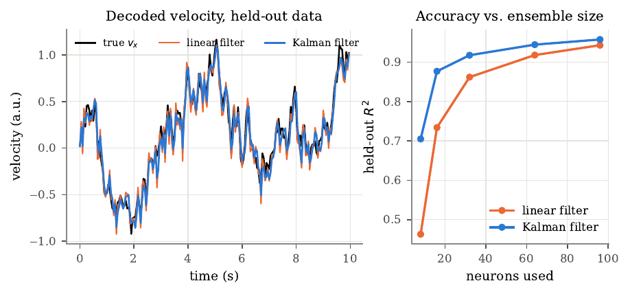
Figure 3. Linear filter versus Kalman filter on simulated data. Two-dimensional velocity follows a smooth random walk, and 96 neurons are linearly tuned to it with Poisson-like noise. Left, true and decoded horizontal velocity on held-out data; the linear filter decodes each 50 ms bin independently and is noisier. Right, held-out \(R^2\) against the number of neurons used. With 96 neurons the linear filter reaches 0.943 and the Kalman filter 0.957; with 8 neurons the values are 0.463 and 0.705. The Kalman advantage is largest when few neurons are available, as the information form predicts. I ran this sweep to watch that prediction play out.

The ridge penalty has a clean reading through the singular value decomposition. Writing \(\bm{F} = \bm{U}\bm{S}\bm{V}^\top\), the fitted values become \(\bm{F}\hat{\bm{B}}_\lambda = \sum_{j} \bm{u}_{j} \frac{s_{j}^2}{s_{j}^2 + \lambda}\bm{u}_{j}^\top\bm{X}\), so directions with large singular values pass almost unchanged while noise-dominated directions with small singular values shrink toward zero. The penalty trades a small bias for a large reduction in variance and equals a Gaussian prior with variance \(\sigma^2/\lambda\) on each weight, and we choose \(\lambda\) by cross-validation on contiguous blocks of time, because neighboring bins correlate and a random split would leak training information into the test set. At the optimum the error has zero correlation with every feature, the orthogonality principle, which is why the filter needs no encoding model. It extracts all the linearly available information, compensating for clumped preferred directions and subtracting shared noise.

An offline decoder predicts movements after the fact, with the user out of the loop; an online decoder sits in a feedback loop where the user sees and corrects the decoded movement, so offline accuracy predicts closed-loop performance poorly. A decoder with modest offline accuracy can give good control if its errors are visible and correctable, and heavy smoothing that raises offline \(R^2\) can make a cursor too sluggish to stop on a target. User and decoder can also learn together. The ReFIT procedure of Gilja and colleagues retrains the Kalman filter on closed-loop data relabeled by the user’s presumed intention. Assuming the user always intended to move straight toward the target at the decoded speed, it rotates each decoded velocity, \(\tilde{\bm{v}}_{t} = \|\hat{\bm{v}}_{t}\| (\bm{g} - \bm{p}_{t})/\|\bm{g} - \bm{p}_{t}\|\), and refits. The idea that activity recorded during brain control should be paired with inferred intention goes back to Taylor’s coadaptive algorithm, whose update compared each unit’s contribution with the cursor-to-target vector and adjusted the weight to reduce the mismatch, applying large changes only when errors were large and consistent. ReFIT adds a second move, the position-feedback assumption. Because the user can already see the cursor, the procedure sets the uncertainty in the position part of the state to zero at each step, so neural activity informs velocity alone and position comes from integrating velocity. All of these methods train on data the decoder itself produced, so a badly wrong initial decoder yields trajectories from which intention is hard to infer, which is why practical protocols begin with an easier task or a short open-loop calibration and refine in closed loop.

Performance metrics try to express speed and accuracy as one number, and all rest on assumptions BCI tasks often violate. Fitts’ law gives movement time as \(a + b\,\mathrm{ID}\) with index of difficulty \(\mathrm{ID} = \log_{2}(D/W + 1)\) bits, and throughput is \(\mathrm{ID}/\mathrm{MT}\). The Wolpaw information transfer rate treats each selection as one use of an \(N\)-ary symmetric channel. With accuracy \(p\) and errors spread evenly,

\[B = \log_{2} N + p\log_{2} p + (1-p)\log_{2}\frac{1-p}{N-1} \quad \text{bits per selection}.\]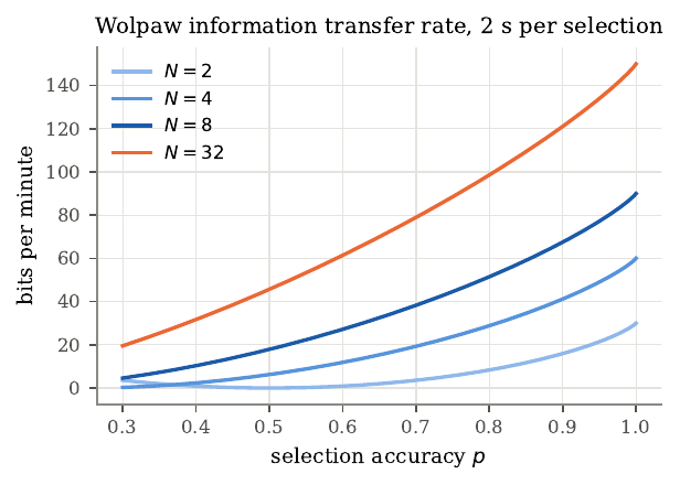

Figure 4. The Wolpaw information transfer rate against selection accuracy \(p\), for 2, 4, 8, and 32 targets at 2 s per selection. At \(p = 0.9\) the rates are 15.9, 41.2, 67.5, and 121.1 bits per minute. The rate is zero at chance accuracy \(1/N\) and rises steeply as accuracy approaches 1, so small accuracy differences among good systems become large rate differences, and more targets give a higher rate at fixed accuracy. Because papers count holds, failures, and target geometry differently, these measures cannot be compared across studies without care.

The three close readings span 23 years and two species and share one argument, that a small sample of motor cortical activity can drive an effector when the user sees the result. Taylor, Helms Tillery, and Schwartz (2002) showed that with about 18 units in monkeys, closed-loop control hit far more targets than the same decoder applied offline, 49 plus or minus 17% of targets in closed loop against 27 plus or minus 9% open loop, all six comparisons significant at \(P < 0.0001\). Tuning changed under brain control, with one unit’s preferred direction shifting by 107 degrees, and coadapted weights, once frozen, generalized to novel targets. Hochberg and colleagues (2006) reported the first BrainGate participant, a man with tetraplegia three years after injury, who controlled a cursor and simple devices from a linear position decoder in primary motor cortex, selecting among 16 targets at 57.8 plus or minus 25.9% correct and among 64 at 16.7 plus or minus 13.2%. The work established that neurons in human motor cortex still modulate with intended movement years after injury, but control was modest, the system needed constant technician tuning, and the accessed text reports no information rate. Shortening the dwell time from 500 to about 250 milliseconds improved success on grids up to 64 targets, which the authors read as the time constraint masking spatial accuracy, a bottleneck in holding still that fits the known weakness of position decoding, in which any noise moves the cursor off target. A 2008 BrainGate follow-up switched to a velocity Kalman filter and found it more accurate, and called the 2006 control insufficiently accurate for many common computer tasks. Willsey and colleagues (2025) decoded four degrees of freedom across three finger groups continuously from the hand knob, using spike-band power and a shallow network retrained with ReFIT-style sign inversion. The participant completed 98.7% of trials at 64 plus or minus 4 targets per minute across all 4D trials, and flew a virtual quadcopter through a 4.5-lap obstacle course, missing 2 of 168 rings. Four-finger control from the hand knob was clean enough to miss only 2 of 168 rings. Adding finger dimensions cost little on the shared fingers, and an offline directional signal-to-noise ratio grew as a power of channel count with exponents of 0.34 to 0.43, below the 0.5 that independent channels would give, and was still rising at 192 channels.

Two details of Taylor’s study matter for the field that followed. In the coadaptive experiments the monkeys’ arms were restrained, and spot checks of muscle activity on well-adapted days showed suppressed electromyography, the paper’s evidence that intention alone drove the control. Frozen weights then generalized to six novel targets, with monkey M hitting 80 plus or minus 26% of novel and 77 plus or minus 24% of trained targets, no significant difference. The paper held the number of units fixed, so its “far fewer cells than expected” rests on offline extrapolations in place of a measured dose-response, and monkey O’s much weaker numbers show that the strongest results came mainly from one animal. Willsey’s study, two decades later, measured the channel scaling directly and found the directional signal-to-noise ratio still rising at 192 channels, and its participation ratio rose to 7.5 with two simultaneous finger targets, 56% above what doubling from the single-target case would predict, a sign that adding dimensions recruits extra neural dimensionality, expanding the space the targets occupy.

The decoders changed in a direction the derivations explain. Taylor used a population vector, Hochberg a position Wiener filter, the 2008 follow-up a velocity Kalman filter, and Willsey a network with 150 ms of history and no explicit dynamics, giving up the Kalman prior for flexibility and relying on closed-loop retraining. Instability links all three. Taylor saw tuning drift, Hochberg recorded 1,536 units from a changing set over 57 sessions, and Willsey’s frozen decoder failed within an hour. Each paper reported its own task and metric, so setting Hochberg’s 16.7% on a 64-target grid beside Willsey’s 64 targets per minute invites a false comparison; part of the gap is progress and part is different tasks, effectors, hold rules, and trial selection. After two decades of progress, recalibration remains necessary, which is why stability deserves its own treatment later in this guide.

Cognitive signals in posterior parietal cortex

The first human BCIs read from primary motor cortex and decoded the moment-to-moment path of a cursor, so a user who wants a cup must steer the hand there continuously. A different strategy reads the goal directly and lets the device plan the path. The evidence for goal signals is strongest in posterior parietal cortex (PPC), which sits between visual cortex and the frontal motor areas and, in monkeys, divides into small areas around the intraparietal sulcus biased toward planning eye movements (LIP), reaches (MIP, the parietal reach region), and grasps (AIP). Human homologues are inferred from fMRI and remain uncertain, so anatomical labels in human studies are hypotheses; the Andersen group later renamed one site PC-IP to describe its location while leaving the monkey homology open.

PPC receives visual input through the dorsal stream, which Goodale and Milner distinguished from a ventral object-recognition stream as mediating the sensorimotor transformations for visually guided action, and it sends output to the frontal premotor areas. Its clinical identity comes from lesions. Patients with parietal damage show optic ataxia, inaccurate visually guided reaching with intact perception, and are selectively impaired at predicting through imagery how long a movement would take, so PPC lesions typically spare strength while impairing the direction and imagination of movement. That pattern made PPC a candidate source of intention signals.

Monkey PPC neurons fire during a delay before a movement in a way that depends on which movement is planned. Snyder and colleagues separated planning from attention by having monkeys plan either a reach or a saccade to one remembered location, and found that delay activity depended on the movement type, which they read as intention. Other groups emphasized that attention strongly modulates parietal responses, and the two views coexist; for a BCI the relevant fact is that delay activity carries information about the planned movement and effector whatever we call it. The prosthetic proposal followed quickly, with Musallam and colleagues decoding movement goals and expected-value signals from monkey PPC, and Mulliken and colleagues showing that PPC activity could also reconstruct continuous trajectories and that many PPC neurons carried a forward estimate of the cursor’s state, consistent with PPC acting as a forward model for online control. PPC also keeps receptive fields fixed on the retina while eye position scales the response, a gain field, modeled as \(r_{i}(x_{r}, e) = f_{i}(x_{r}) g_{i}(e)\). A single gain-field neuron is ambiguous, but a population carries head-centered position implicitly. An additive population \(r_{i} = f_{i}(x_{r}) + g_{i}(e)\) stays additively separable, and a head-centered tuning curve \(h(x_{r} + e)\) has a nonzero mixed partial derivative, so no linear weights produce it. A multiplicative population escapes this. Summing Gaussian gain-field neurons along the line \(a + b = c\) gives a downstream response

\[R_{c}(x_{r}, e) = \sqrt{\pi\sigma^2}\,\exp\!\left(-\frac{(x_{r} + e - c)^2}{4\sigma^2}\right),\]

tuned to the head-centered position \(x_{r} + e\). Products of functions of \(x_{r}\) and functions of \(e\) can approximate any continuous function of the pair (Stone-Weierstrass), which is the basis-function view of Pouget and Sejnowski. A ridge readout of a simulated multiplicative population reached a held-out \(R^2\) of 0.996 to 0.997, while the additive population reached only 0.24 to 0.27. I built both populations to test this, and the separation was total, with the multiplicative code almost perfectly readable and the additive one barely above a quarter. This basis-function idea extends. Products of functions of the two inputs can approximate any continuous function of the pair, and gain-field-like units emerge naturally when a network learns to compute spatial location, though it leaves open whether the brain learns them the same way. PPC also appears to code reach plans in eye-centered coordinates, which is one reason gaze and hand stay coordinated, since in natural tasks people look at where the hand is going and hold gaze on the target of a reach. For a BCI this matters because if PPC codes goals relative to gaze, a decoder trained while the user fixates one point may misread goals when the user looks elsewhere, so a system that tracks gaze and uses it as signal might do better. People with tetraplegia usually retain their eye movements, so gaze is both a confound to control and a signal a decoder could exploit.

Goal and trajectory decoding are complementary. A goal decoder classifies neural activity into one of a finite set of targets from planning activity, so it is fast but needs a known target set and locks in once it classifies; a trajectory decoder works in open space and allows continuous correction but is slower. They can combine. If a goal decoder supplies a prior \(\pi_{0}(g)\) and the trajectory decoder produces noisy velocity estimates, the posterior over targets after \(t\) bins is \(\Pr(g \mid \bm{n}, \bm{y}_{1:t}) \propto \pi_{0}(g)\prod_{s} p(\bm{y}_{s} \mid g)\). The log odds against a competitor drift upward at rate \(D = v^2\|\bm{\Delta}\|^2/(2\sigma^2)\), the Kullback-Leibler divergence per bin, from a starting value \(\Lambda_{0} = \log[\pi_{0}(g^*)/\pi_{0}(h)]\), so with a selection threshold \(A\) the expected decision time is

\[t^* \approx \frac{A - \Lambda_{0}}{D}.\]

The prior and the trajectory evidence are interchangeable. One nat of prior log odds saves the time needed to accumulate one nat of evidence. A worked example with six targets shows a confident goal decoder (0.8 on the correct target) cutting decision time by about 65%. But the benefit depends on calibrated probabilities; a confidently wrong prior makes the combined system worse.

Aflalo and colleagues (2015) reported the first recordings from microelectrode arrays in human PPC, in a man paralyzed for ten years, with arrays in putative area 5d and putative AIP targeted by fMRI of imagined reaching and grasping. He could modulate individual neurons by imagining specific actions with no visual stimulus present, which argues against a purely attentional account. A masked memory reach task separated goals from trajectories. Of 124 spatially tuned units, 19% coded the goal only, 54% the trajectory only, and 27% both, an early human example of mixed selectivity. A classifier decoded goal identity from delay-period activity above 90% using fewer than 30 units, with goal information significant within 190 ms of the cue. Fewer than 30 parietal units carried a goal this clearly, before any movement began. Individual neurons preferred imagined right-arm reaches, imagined left-arm reaches, or saccades, with preferences intermixed on single arrays, and many reach-selective neurons were bimanual. The headline accuracy comes from units selected greedily and pooled across days, so it is optimistic for real-time use, and there is one participant. A control also mattered. Goal decoding was similar whether a flash cued the target directly or a symbol on a grid did, which argues the signal reflects the intended goal more than the visual input, though a symbolic cue still specifies a location the participant could image. The effector analysis found the population biased toward reaches and, for the right-versus-left comparison that avoids the imagined-versus-actual confound, many bimanual reach neurons, suggesting that independent control of two arms from PPC may be hard.

A distinction the human studies force is between motor imagery and attempted movement. In a person with a complete spinal cord injury both stay silent, and from the outside the two look alike, but they are different instructions, and a decoder calibrated on one may degrade when the user switches. Aflalo asked his participant to imagine movements, while Guan asked hers to attempt finger presses as though pressing a key, so their accuracy figures resist direct comparison. The Andersen group has shown that strategy can itself be a coded variable in anterior intraparietal cortex, which argues for holding the strategy fixed between calibration and use or training across strategies.

Two later papers from the same program extended the picture. Guan and colleagues decoded individual fingers from PC-IP at 86% online across ten sessions with gaze controlled, with a muscle-like representational component emerging 170 ms before a somatotopic one, consistent with a forward model; and Chivukula and colleagues decoded felt and observed touch (discussed elsewhere in this guide). The human recordings depart from the monkey picture of anatomically separate effector areas, finding effector preferences intermixed and finger coding at a site originally targeted as a grasp area, though species, imprecise homology, and the move to imagined movement could each contribute. The goal-versus-trajectory theory suggests a hybrid decoder using goal activity as a prior on trajectory decoding would have the most to gain where Aflalo found both signals in the same 27% of neurons, if the goal probabilities are well calibrated, which published goal-decoding studies rarely measure. The same planning signals can also be reached less invasively with functional ultrasound, taken up at the end of this guide.

Recording modalities and the engineering of a sensor

Every BCI begins with a sensor that converts the electrical activity of neurons into a measurable voltage, and that choice fixes what every later stage can use. A neuron generates extracellular potential by passing current across its membrane into the conducting tissue. Treating the tissue as a purely resistive medium, a point current source \(I\) at the origin satisfies Poisson’s equation \(\nabla^2 V = -(I/\sigma)\delta(\bm{r})\), and by Gauss’s theorem all the injected current crosses a sphere of area \(4\pi r^2\), so the potential is

\[V(r) = \frac{I}{4\pi\sigma r}.\]

An actual neuron’s currents sum to zero, so its simplest far field is a dipole whose potential falls as \(1/r^2\), and quadrupoles fall faster still. This is why a microelectrode records spikes only from a small neighborhood and why the neurons it records can change when the tip moves by tens of micrometers. It is also why scalp EEG exists at all. Pyramidal neurons are aligned in parallel, and when many receive synchronous input their dipoles add into a large one that distant electrodes can see, while asynchronous, sparse activity such as individual action potentials nearly cancels. The skull, far less conductive than brain or scalp, spreads the current laterally and blurs it over centimeters. Different frequency bands reflect different processes. Spikes (hundreds of hertz to kilohertz) need proximity, high-gamma power (about 70 to 150 Hz) correlates with local population firing and falls off quickly, and slow rhythms survive to the scalp. Each modality is a different answer to how many tissue layers to cross. Scalp EEG crosses all of them and is blurred; ECoG sits on the cortex under the dura; stereo-EEG reaches deep structures through drill holes; endovascular arrays sit inside veins; penetrating Utah arrays enter the cortex and record spikes at the cost of a percutaneous connector and a foreign-body response that encapsulates the electrode over months.

That foreign-body response bears on recording quality in a way the physics makes concrete. An acute phase follows the insertion injury, and a chronic phase leaves activated microglia and a sheath of reactive astrocytes, the glial scar, which raises the electrode’s impedance. Comparisons of implanted electrodes against stab wounds made by the same devices and immediately withdrawn associate persistent inflammation and neuron loss with the continued presence of the device, beyond the insertion injury alone. Because a recorded spike falls off so steeply with distance, losing the neurons within the closest tens of micrometers removes the cells that produced the largest signals, which plausibly contributes to the slow changes in recorded signals over months and years documented in macaque motor cortex. For an endovascular stent the vessel’s inner lining gradually covers the device over about 45 days, a process that limits chronic recording while still allowing it, with reported thrombosis or hemorrhage rates below 0.5% for stents in comparable veins.

Even the quietest electrode has a noise floor. Any resistance at temperature \(T\) generates Johnson-Nyquist noise, which Nyquist derived from thermal equilibrium on a transmission line. Each electromagnetic mode carries average energy \(kT\), and matching the delivered power \(kT\,\Delta f\) to that of a noisy resistor driving a matched load gives

\[v_{\mathrm{rms}} = \sqrt{4kTR\,\Delta f}.\]

For a 1 megohm electrode recorded over 10 kHz at body temperature this is about 13 microvolts, a central concern for microelectrodes; for a 10 kilohm scalp electrode over 100 Hz it is about 0.13 microvolts, two orders of magnitude lower, so muscle and environmental artifacts set EEG’s floor. A decoder works from features computed from the raw voltages. One is threshold crossings (a spike is marked when the filtered signal falls below \(-k\sigma\), with the noise level estimated as \(\hat\sigma = \mathrm{median}(\vert x\vert )/0.6745\), since the median ignores the rare large values spikes produce); another is band power computed with Welch’s method, which averages \(K\) windowed periodograms to cut the periodogram’s variance, which otherwise equals its own mean regardless of record length. The choice of threshold trades missed spikes against false detections, and Rice’s formula gives the false-crossing rate from Gaussian noise, which for a 300 Hz to 6 kHz band falls from about 39 per second at \(k = 3\) to about 0.14 per second at \(k = 4.5\). Many human intracortical BCIs feed the decoder unsorted threshold crossings in place of spike-sorted units, because sorting needs stable waveforms that chronic arrays often lack, which is itself a stability problem.

Schalk’s capacity argument rests on Shannon. A channel adding Gaussian noise of power \(N\) to a signal of power \(S\) over bandwidth \(B\) has capacity \(C = B\log_{2}(1 + S/N)\), and \(M\) independent channels add. Schalk’s 2008 perspective frames the problem as a communication bottleneck. The brain has great computational breadth but little serial depth, the computer the reverse, and a narrow, slow channel of speech, typing, and pointing joins them, stripping the brain’s semantic context into mere keystrokes. He argued that BCI information rate grows with the number of independent channels and the clarity of each, and concluded that the sensors, more than the algorithms, were the main bottleneck. He distinguished using the brain’s existing language from establishing a new one, listed the reference problem (decoders need an observable reference to calibrate against) and non-stationarity (symbols drift over time) among the obstacles, and worked through a hypothetical 1,000-channel wireless implant to show that telemetry links lack the bandwidth for raw broadband data, so implants must compute features on-device. His central claim, that sensors are the bottleneck, has held in the specific sense that the largest gains since 2008 have come from recording more neurons more closely, while his forecasts of adoption by healthy users have fallen short. Willsey’s channel-count result, with its sub-ideal exponent, both supports his prediction that more channels help and shows the gain is smaller than independent channels would give.

Oxley and colleagues (2020) tested the opposite extreme, how little invasiveness a useful home system needs. Two people with ALS received the Stentrode, a 16-electrode array on a stent delivered through the jugular vein into the superior sagittal sinus, with fully implanted wireless telemetry sealed beneath the skin. A decoder detected attempted movement versus rest from normalized band power (mu and beta for one participant, extending toward high gamma for the other), and timing logic turned that single binary signal into clicks, while an eye tracker moved the cursor. Both typed with click-selection accuracy above 92%, at 13.81 and 20.10 correct characters per minute, ran the system at home on their own, and had no serious adverse events over the reporting period. The neuroprosthesis-alone information transfer rates of 0.32 and 0.46 bits per second fall in the same range as the 0.41 bits per second Schalk cited as the 2008 BCI ceiling, so the ceiling moved little in twelve years, while the setting changed completely. Across these two papers, the information rate barely moved while the device went from a lab rig to something a person runs at home. The device ran at home, fully implanted and wireless. Stability and information per channel appear to trade against each other across modalities, since the coarse field-potential signal needed almost no recalibration, and its cost was a low rate. We can explain the Stentrode result from the physics. The array sits beneath the skull, so it escapes the blurring that limits EEG, but it is farther from neurons than an ECoG electrode, so by the inverse-distance law it integrates over a larger volume, and its signal content, mu and beta power with some reach toward high gamma, matches that position. The final trial report describes offline decoding of at least five attempted movement types, with a mean signal bandwidth of 233 Hz stable over the study, but whether multiclass decoding holds up online, over months, and at home is unreported, and the superior sagittal sinus lies over the leg area, so reaching the hand area would need a different vein.

Plasticity and stability

A BCI learns a mapping from neural activity to intended behavior on one day and bets it will hold tomorrow. Three different things can break that bet, and confusing them is easy. Representational stability concerns whether the same intention evokes the same population pattern over time; recording stability concerns whether each channel measures the same source, which intracortical electrodes violate routinely as the tip moves and neurons die or get encapsulated; decoder stability concerns whether the output stays accurate under a fixed fit. Evidence about one kind stays specific to it. A recording can drift while the representation stays the same, a representation can stay stable for the weeks of a study after reorganizing in the years before, and changes elsewhere in the pathway can generate what we measure in cortex. The field’s remedies divide along the same lines. Supervised recalibration refits the decoder with new labeled data; self-recalibration infers the user’s intended movement during free use and refits on those inferred labels, as ReFIT does; and unsupervised alignment leaves the decoder fixed and transforms new neural data to resemble the training data, which is the approach the stabilizer below takes.

Pons and colleagues (1991) asked how far the adult somatosensory map can change after long-term loss of input. Earlier nerve-cut experiments had found reorganization over only one to two millimeters, which fit the spread of thalamocortical branches. In macaques whose sensory roots for one arm had been cut more than a decade earlier, the deprived hand-and-arm territory came to respond to touch on the face, a change later quantified as going from one to two millimeters to about 10 to 14 millimeters, an order of magnitude larger than anyone expected and far beyond what unmasking existing inputs could explain. (I had only the abstract and secondary sources.) Where the reorganization happens became the central debate. Later work found severe transneuronal atrophy and map expansion in the brainstem cuneate nucleus and thalamus, intracortical sprouting, and, most directly, that inactivating the reorganized cuneate nucleus made the expanded face representation in cortex disappear. A later reappraisal by Makin and Bensmaia argued that for human amputees the phrase “massive reorganization” overstates the case, and that the original limb representation largely survives beneath new inputs. This bears directly on BCIs, because stimulation of S1 in people with spinal cord injury evokes sensations felt on the hand, and motor cortex still contains hand-tuned neurons years after injury, both hard to reconcile with a complete takeover.

Guan and colleagues (2022) addressed the question quantitatively, in a woman with tetraplegia ten years after a C3-C4 injury, whose PC-IP array decoded attempted finger presses. To compare representations across people and methods at the population level, they used the cross-validated Mahalanobis distance. Naive squared distances are biased. \(\mathbb{E}[\|\hat{\bm{b}}_{j} - \hat{\bm{b}}_{k}\|^2] = \|\bm{b}_{j} - \bm{b}_{k}\|^2 + (2/n)\operatorname{tr}(\bm{\Sigma})\), so noise always inflates them. Estimating the two difference vectors from independent partitions removes the bias, since \(\mathbb{E}[\hat{\bm{\delta}}_{A}^\top\hat{\bm{\delta}}_{B}] = \|\bm{b}_{j} - \bm{b}_{k}\|^2\), and the resulting “crossnobis” distance can be negative when two conditions are identical, which makes it safe for testing change over time. An online decoder classified finger presses at 86% plus or minus 4% (chance 17%), 89% of neurons were tuned, and the representational geometry matched able-bodied fMRI, the participant’s dissimilarity matrix being statistically typical of 36 able-bodied participants. The geometry held steady over six weeks of BCI use, with session-to-session correlations of \(r = 0.90\) plus or minus 0.04 and Bayes factors favoring no change. A time-resolved analysis found a muscle-like component emerging 170 ms before a somatotopic one, consistent with a forward model. The study establishes only that the representation is stable now and able-bodied-like, leaving open whether it stayed the same during the decade after injury, and the title was changed from “Preserved” to “Stability of motor representations after paralysis” in review to reflect this caution.

Degenhart and colleagues (2020) attacked recording instability directly. Population activity often lies on a low-dimensional manifold, and factor analysis (FA) separates shared variance from private noise. With latent \(\bm{z}_{t} \sim \mathcal{N}(\bm{0}, \bm{I})\) and \(\bm{u}_{t} \mid \bm{z}_{t} \sim \mathcal{N}(\bm{\Lambda}\bm{z}_{t} + \bm{\mu}, \bm{\Psi})\) and diagonal \(\bm{\Psi}\), the marginal covariance \(\bm{\Lambda}\bm{\Lambda}^\top + \bm{\Psi}\) splits into a low-rank shared part and a diagonal private part, which distinguishes FA from PCA, where a single noisy electrode can dominate a component. FA is identifiable only up to rotation, since replacing \(\bm{\Lambda}\) with \(\bm{\Lambda}\bm{O}\) for any orthogonal \(\bm{O}\) leaves the marginal unchanged, so two sessions describe the same manifold with differently rotated axes. The orthogonal Procrustes problem resolves this. The rotation minimizing \(\|\bm{X} - \bm{Y}\bm{O}\|_{F}^2\) is \(\hat{\bm{O}} = \bm{U}\bm{V}^\top\) from the SVD of \(\bm{Y}^\top\bm{X}\). The stabilizer fits a new FA model to recent data, finds the electrodes whose relationship to the manifold held steady with a greedy residual procedure, aligns the new loadings to the old ones on those stable electrodes, and feeds the aligned latents to a fixed decoder. In two monkeys, after deliberately severe induced instabilities, it restored the success rate to 98.3 plus or minus 0.4% against a 99.9% baseline, recovered within about one update (89 seconds of control time), and improved performance in 38 of 42 experiments while leaving the rest unchanged. I read this as the strongest case in the guide for working at the level of the population, since the alignment rides on the covariance structure alone. Manifolds fit right after an instability still captured 76 plus or minus 2% of the baseline shared variance, against 17% for random manifolds, confirming the premise. An offline comparison against recalibration that used the true intended direction, an upper bound on intent-based self-recalibration, is telling. In the brief window at the start of each trial when directional information is weakest, the stabilizer reduced angular error by 20.2 degrees on average against recalibration’s 5.7, because recalibration needs clear directional information while the stabilizer needs only the covariance structure. The recovery was partial, since the stabilized acquisition rate stayed below baseline, and the shortfall tracked how much target information survived the instability, more than the number of dropped electrodes. The instabilities were imposed artificially and chosen to be severe, and the tuning-change instability substituted neurons from the same array, which belong to the same manifold and so favor alignment. Factor analysis also treats each time bin independently, a limit the later NoMAD method addresses by aligning latent dynamics models, connecting this problem to the dynamics methods in the next section.

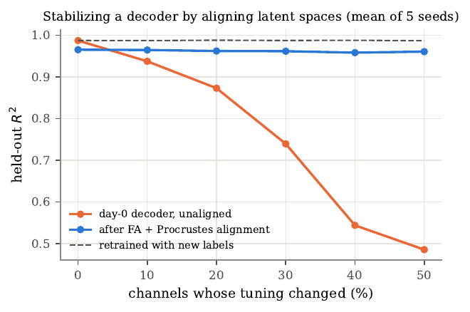
Figure 5. Simulated decoder stabilization. A day-zero decoder applied to later data without alignment (upper curve degrading) falls from \(R^2 = 0.99\) to 0.49 as half the channels change their tuning. Fitting new factor-analysis parameters and aligning them to the day-zero loadings with orthogonal Procrustes on automatically identified stable channels keeps performance near \(R^2 = 0.96\), close to a decoder retrained with ground-truth labels. Means over five seeds. The method recovers less if the manifold itself drifts, since here the changed channels received loadings on the same latent manifold.

The three papers answer different questions, and together they sharpen each other. Pons measured which body part drives neurons in a deafferented sensory map; Guan measured the relational structure of attempted movements in an association area that still receives intact motor-planning input. New inputs can invade a sensory map while the motor intentions represented nearby persist. Guan and Degenhart share a stance. Both compare populations as a whole, because population-level structure is more stable than its components, a point later documented over two years in monkeys. The practical lesson is that representations in current BCI targets are stable enough over months to support long-term decoding, recording instabilities are the larger day-to-day problem and can be handled by unsupervised alignment, and learning is either a problem or a resource depending on whether the decoder is perturbed.

Neural population dynamics and latent variable models

A motor BCI receives a new vector of spike counts every few tens of milliseconds, and each entry is sparse and noisy; in a 10 ms bin a cortical neuron usually stays silent. Classical neurophysiology removed this noise by averaging over many repeats of the same condition, but a BCI must act on the trial in progress. The idea developed here treats the population as a dynamical system, so that activity at one moment constrains the next and each noisy bin borrows information from its neighbors in time. Under the dynamical systems view, population activity is the state of a system evolving by its own rules, \(\bm{x}_{t+1} = f(\bm{x}_{t}) + \bm{u}_{t}\), with inputs \(\bm{u}_{t}\) from outside the modeled population. Linearizing near a fixed point gives \(\bm{x}_{t+1} = \bm{A}\bm{x}_{t}\), whose modes rotate and decay by the eigenvalues of \(\bm{A}\); a skew-symmetric continuous-time generator produces pure rotation, since \(\frac{d}{dt}\|\bm{x}\|^2 = 2\bm{x}^\top\bm{M}\bm{x} = 0\). Churchland and colleagues found this rotational structure in condition-averaged motor cortex with jPCA, with different reach conditions starting from different points in a plane and rotating in the same sense, as a single dynamical system acting on condition-specific initial states would. Under this view the preparatory activity before a movement sets the initial state, the dynamics then generate the movement, and inputs enter only for surprises beyond the initial state, such as an unexpected cursor jump. For decoding the practical consequence is a prior. Knowing the dynamics lets us predict the next state and weigh a noisy observation against that prediction, so a dynamics model removes noise by exploiting temporal structure within one trial the way trial averaging removes it by exploiting repetition.

The linear Gaussian state-space model is factor analysis with memory, and every result follows from one fact. For jointly Gaussian \((\bm{a}, \bm{b})\), the conditional \(\bm{a} \mid \bm{b}\) is Gaussian with mean \(\bm{\mu}_{a} + \bm{\Sigma}_{ab}\bm{\Sigma}_{bb}^{-1}(\bm{b} - \bm{\mu}_{b})\) and covariance \(\bm{\Sigma}_{aa} - \bm{\Sigma}_{ab}\bm{\Sigma}_{bb}^{-1}\bm{\Sigma}_{ba}\). Applying it forward gives the Kalman filter; applying it backward through the Markov structure gives the Rauch-Tung-Striebel smoother, which corrects each filtered estimate by how much the future revised the next-step prediction. The smoother is acausal, which is why its estimates beat the filter’s and why it runs only offline. We learn the parameters of a linear dynamical system with expectation maximization, where the E-step runs the smoother and the M-step updates each parameter by a regression that replaces outer products of latents with their posterior expectations. The model is identifiable only up to an invertible linear transform of the latent, which fixes the eigenvalues of the dynamics matrix, hence the frequencies and decay rates of the latent modes, but leaves the coordinate axes free, so “latent dimension 1” means something across two fits only after alignment. Gaussian-process factor analysis imposes temporal smoothness a different way, placing a smoothness-kernel prior on each latent independently, but because its dimensions are independent a priori it treats a peak in one dimension and a quarter-cycle-later peak in another as unrelated, where a rotation couples them; it imposes smoothness and leaves dynamics out.

Spike counts follow Poisson statistics, so we either keep a Poisson observation model \(y_{n,t} \sim \mathrm{Poisson}(\exp(\bm{c}_{n}^\top\bm{x}_{t} + d_{n}))\), whose log posterior is concave but no longer closed-form, or variance-stabilize with a square-root transform, since \(\mathrm{Var}[g(y)] \approx g'(\lambda)^2\lambda\) is constant when \(g(y) \propto \sqrt{y}\), and the Anscombe form \(\sqrt{y + 3/8}\) improves the approximation at low counts.

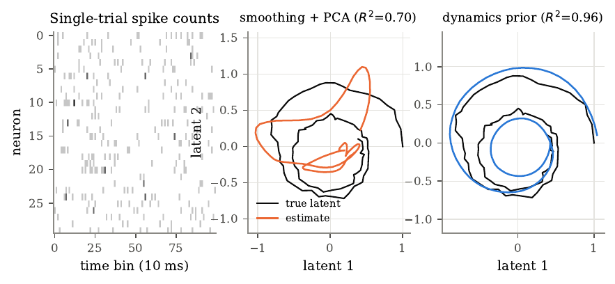
Figure 6. A dynamics prior recovers single-trial latent structure. Left, spike counts of 30 of 50 simulated neurons in one trial of 100 bins, driven by a two-dimensional damped rotational latent through log-linear Poisson tuning; by eye the trial is nearly featureless. Middle, the true latent and the estimate from Gaussian-kernel smoothing plus PCA, mapped to the truth by a least-squares affine fit (\(R^2 = 0.70\)). Right, the estimate from a Rauch-Tung-Striebel smoother on square-root transformed counts using the known dynamics (\(R^2 = 0.96\)). The dynamics prior lets all 100 bins inform the estimate at each one, rejecting noise that does not fit any allowed trajectory. The smoother here was given the true dynamics and an oracle readout, so the figure isolates a mechanism rather than estimating average performance.

Once the dynamics are a learned nonlinear network and the observations Poisson, the posterior loses its closed form, and variational inference replaces it with a tractable approximation. Introducing any distribution \(q(\bm{z})\) and applying Jensen’s inequality gives the evidence lower bound (ELBO), \(\log p_\theta(\bm{y}) \ge \mathbb{E}_{q}[\log p_\theta(\bm{y}\mid\bm{z})] - D_{\mathrm{KL}}(q \,\|\, p(\bm{z}))\), and the gap between the two is \(D_{\mathrm{KL}}(q \,\|\, p_\theta(\bm{z}\mid\bm{y}))\), so maximizing the ELBO over \(q\) makes \(q\) as close as possible to the posterior. The reparameterization trick writes a Gaussian sample as \(\bm{z} = \bm{\mu}_\phi + \bm{\sigma}_\phi \odot \bm{\epsilon}\) so the gradient passes inside the expectation, where an alternative score-function estimator would have far higher variance, and a variational autoencoder (VAE) trains an encoder network to output the posterior parameters for each data point, amortizing the cost of inference so a new point needs only one forward pass. A powerful decoder can sometimes model the data while ignoring the latent, and the optimizer then drives the approximate posterior to the prior to remove the KL penalty, a failure called posterior collapse, which LFADS guards against by raising the weight on the KL term from zero over the first couple of thousand training steps so the encoder learns to use the latents before it pays full price for them.

LFADS, from Pandarinath and colleagues (2018), is a sequential VAE whose decoder is a recurrent network acting as a learned dynamical system. It represents each trial by an initial condition \(\bm{g}_{0}\), evolves a generator RNN under optionally inferred inputs \(\bm{u}_{t}\), projects the state to low-dimensional factors, and reads out Poisson rates. In the autonomous case the whole trajectory is a function of \(\bm{g}_{0}\) alone, so the encoder must compress the entire trial into one vector that the learned dynamics can turn back into a trajectory, which is how the dynamics prior enters. On monkey motor-cortex data its rates decoded hand velocity at \(R^2 = 0.90\), against 0.66 for Gaussian smoothing and 0.69 for GPFA, and it needed only 25 to 50 neurons to beat those methods using all 202, which I found the most convincing number in the paper, since it is the empirical form of the information-form argument I had just derived for the Kalman filter. the empirical counterpart of the information-form argument. It revealed rotational dynamics on single trials for the first time, inferred inputs that tracked unexpected cursor jumps, and, through multi-session “stitching” with per-session linear read-in and read-out maps, supported one decoder across 44 sessions over 162 days with entirely different neurons. The authors caution that the generator is an abstract device far from cortical biophysics, and that separating inferred inputs from dynamics is ill-posed, since reconstruction quality cannot settle it. The controller that infers inputs plays the part of process noise, receiving the generator’s previous factors so it knows what the generator is about to do, and the inferred input is close in spirit to the Kalman innovation, the residual the dynamics leave behind, except that it passes through a KL penalty and a few dimensions before it can act. Two mechanisms limit how much information flows through it, the KL penalty and a small input dimension; with those limits removed, the controller could transmit the data directly and the generator would skip learning dynamics. The methods of this section form a ladder of assumptions about the hidden state. Factor analysis assumes a low-dimensional state but no memory, GPFA adds smoothness, the linear dynamical system adds linear dynamics that couple dimensions, and LFADS keeps the Poisson likelihood while learning nonlinear dynamics and paying for both with amortized variational inference. Each step trades bias for variance, giving less noise when the structure is right and systematic error when it is wrong.

Stitching and the Degenhart stabilizer rest on the same premise, that recorded neurons are changing views of a latent system that stays the same; Procrustes alignment resolves the rotational ambiguity by matching loadings, and stitching resolves the larger linear ambiguity by forcing all sessions through one generator. The velocity Kalman decoder of the motor section and LFADS apply the same predict-update idea at different places, one to the cursor’s state and one to the neural state, and a decoder taking LFADS factors as input would combine two dynamics priors, though doing it online needs a causal encoder the original model lacks.

Writing to the brain, restoring touch

Every interface so far reads the brain. Restoring touch means writing into it. After a spinal cord injury, the pathway carrying the arm’s signals to cortex is cut, so intracortical microstimulation (ICMS) passes small currents through penetrating electrodes in primary somatosensory cortex (S1), and when the electrode lies in the hand representation the person feels a sensation on the hand. Touch matters for dexterity because grasping depends on fast signals about contact and slip that only touch supplies. Johansson’s classic work showed grip force rising in parallel with load force, adapted to surface friction within about 0.1 second of contact, and this adaptation depended on cutaneous input. A simple control model shows why slow feedback makes control slow. If a controller corrects an error at rate \(K\) but only learns it after delay \(\tau\), the characteristic equation \(s + Ke^{-s\tau} = 0\) has its stability boundary at \(K_{\max} = \pi/(2\tau)\), so doubling the delay halves the fastest stable correction. A BCI user relying on vision alone must handle every surprise through it, with longer delays, and should be slowest where force must be adjusted, which is the grasp. The model is a caricature, because actual motor control combines feedback with prediction through internal models, but prediction helps only when the world behaves as expected and breaks down when an object is heavier or more slippery than predicted, the case where touch triggers its fast corrections. In the Flesher system the sensor-to-stimulation path took under 20 milliseconds, while the cortical part of the delay went unmeasured.

ICMS delivers brief charge-balanced biphasic pulses, and two quantities govern safety, the charge per phase \(Q = I\,t\) and the charge density \(D = Q/A\). The Shannon model fits a line through tissue-damage data, \(\log_{10} D = k - \log_{10} Q\), so \(k = \log_{10}(Q \cdot D)\) and the largest safe charge grows only as the square root of electrode area, \(Q_{\max} = \sqrt{A \cdot 10^k}\). Investigators usually take \(k\) between 1.5 and 2.0. The model was built for macroelectrodes, and direct tests show microelectrodes can be damaged well below the \(k = 1.85\) line, so the Shannon line falls short as a safety argument for human ICMS. Current spread follows the point-source potential, and the current needed to activate a neuron grows roughly as the square of distance, \(I = Kr^2\), with \(K\) between about 100 and 4000 microamps per square millimeter, so the activated volume grows as \(I^{3/2}\). For the 64 microamp maximum in Flesher, this gives an effective radius between about 0.13 and 0.8 mm depending on the excitability constant, and since the activated volume grows as the three-halves power of current, doubling the current activates almost three times as much tissue, enough that neighboring electrodes 0.4 mm apart overlap across most of the plausible range. But imaging shows a sparse, distributed pattern, because stimulation mostly activates axons passing within tens of micrometers of the tip regardless of the cell body’s location, so ICMS recruits neurons regardless of their feature selectivity. In area 1 the neurons near an electrode share a rough location on the hand, because the somatotopic map is orderly, but they may differ in preferred orientation or motion direction, which is the non-specific activation the patterned-stimulation study identifies as a core limitation. The percept is felt at a projected field on the body, whose location follows the somatotopic map and is stable over months, and overlapping fields from several electrodes combine roughly additively into more localizable, more intense sensations.

The hand’s glabrous skin carries four classes of mechanoreceptive afferent, named by how they respond to sustained indentation and by receptive-field size. Slowly adapting type I afferents (Merkel) signal sustained pressure and fine spatial detail, rapidly adapting type I (Meissner) respond to changes and small slips, slowly adapting type II (Ruffini) respond to skin stretch, and rapidly adapting type II (Pacinian) are extremely sensitive to high-frequency vibration transmitted through a held object. Slowly adapting afferents report how hard and where, rapidly adapting ones report that something has changed. Their signals reach four subdivisions of S1 across the central sulcus, with receptive fields growing and selectivity becoming more complex from area 3b to 1 to 2. Area 3b would offer the smallest receptive fields but lies deep in the sulcus, so both studies here implanted area 1, whose neurons show tuning for edge orientation and motion, the signal patterned multi-electrode stimulation might exploit. The encoding, the map from sensor reading to stimulation, is a design choice. Flesher’s linear scheme maps force to amplitude and, with a just-noticeable difference near 15 microamps over a 50 microamp range, supports about four distinguishable levels, enough to say light or firm and too few for fine gradations. A biomimetic scheme adds a term proportional to the rate of change of force, imitating the transient on and off responses of natural afferents, which in human tests feels more like an actual indentation on more electrodes and disturbs the motor decoder less.

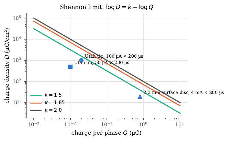
Figure 7. The Shannon model of stimulation safety. Lines show \(\log_{10} D = k - \log_{10} Q\) for \(k = 1.5\), 1.85, and 2.0, with charge density \(D\) and charge per phase \(Q\) on logarithmic axes; points below a line are predicted safe for that \(k\). Two example points represent a Utah array electrode tip at 100 and 50 microamps for 200 microseconds, and a third a 2.3 mm surface disc at 4 mA. The tip area is an assumption for illustration, not a measured value, and the Shannon model, built from macroelectrode experiments, is debated for penetrating microelectrodes.

Flesher and colleagues (2021) built a bidirectional BCI with motor arrays for decoding and area 1 arrays for stimulation, driving five electrodes from two torque sensors on a robot hand with a linear encoding that mapped torque to amplitude (14 to 64 microamps). The participant, who could still see, completed a modified clinical arm test with a median score of 21 with ICMS against 17 without, and median trial time fell by half, from 20.9 to 10.2 seconds. The improvement concentrated in the grasp phase, which fell 66% and accounted for 88% of the total gain, as the feedback-delay argument predicts. The gain landed almost entirely in the grasp, the one phase where my simple delay model says touch should matter most. The number of successful trials held constant, so ICMS made the participant faster while leaving his success rate the same, and the benefit appeared from the first session. There was one participant over four sessions per condition, no sham condition, and the participant knew when ICMS was on, so confidence and sensory information stay entangled.

Valle and colleagues (2025) asked whether stimulation can carry more than location and intensity. Stimulating groups of area 1 electrodes whose projected fields traced lines, they evoked oriented edges; stimulating them in sequence evoked apparent motion. In forced-choice tasks, participant c1 recognized edge orientation at 81 to 89% across digits, recognized objects (pen, can, ball) at 79 plus or minus 11%, and recognized directions of motion at 76 to 98%, with recognition insensitive to amplitude (so the identity of the active electrodes carried the structure) and dependent on train duration. Apparent motion appeared only when successive trains were separated by 0 to 0.5 seconds. Speed discrimination reached a Weber fraction of 0.56, within the range of natural touch. In a closed-loop test c1 steered a robot arm guided only by ICMS motion cues, at 85 plus or minus 9% with no added load. Many headline findings came from one participant, c2’s shape recognition was much weaker, and accuracy was tested against chance task by task with no correction for multiple comparisons. Valle also conveyed curvature by raising the amplitude of a central electrode relative to its flankers and starting it earlier, with c1 recognizing concave, flat, and convex stimuli at 64 plus or minus 7%, and conveyed motion equally well by current steering, varying the relative amplitudes of three adjacent electrodes to slide the active peak. The window for perceiving continuous motion was the same 0 to 0.5 seconds between trains, independent of how far apart the fields lay, so the percept depends on timing, more than on spatial separation. Sequentially traced letters beat letters stimulated all at once, and the sequential advantage grew with letter complexity, a direct parallel to dynamic stimulation of visual cortex.

The two papers suggest a division of labor echoing the mechanoreceptor classes. Flesher’s sustained pressure signal imitates slowly adapting afferents, Valle’s sequential patterns the rapidly adapting ones, though each delivers one class at a time in a manipulation task, and both leave the biomimetic onset and offset transients aside. Both depend on the persistence of the hand map after injury, in participants who had lived ten and thirty-five years with their injuries, which argues against a complete takeover of the hand territory, though each of these injuries spared some sensation, so the map’s survival after a complete sensory injury remains untested. Both confront the central problem of bidirectional BCIs, that writing interferes with reading. Flesher’s system blanked and filtered stimulation artifacts, Valle’s held the decoder fixed during stimulation, and the interference runs deeper than artifacts, because stimulation of S1 evokes activity in motor cortex that a decoder trained in its absence may misread. As feedback grows richer and uses more electrodes at higher amplitudes, both the interference and the question of safety at scale, which the Shannon line cannot settle for microelectrodes, grow with it.

Restoring sight and hearing

A sensory prosthesis takes a signal from a camera or microphone and writes it into the nervous system as electrical stimulation, so that the brain may treat it as sight or sound. Writing is harder to evaluate than reading, because an evoked percept exists only in the user’s report, so every experiment here rests on psychophysics. The two senses have had different histories. The cochlear implant is the most widely used neural prosthesis, with about one million users who on average understand most sentences in quiet; visual prostheses have reached far fewer and restore far less. Part of the reason is dimensionality, since the cochlea lays out frequency along a line while primary visual cortex lays out a two-dimensional field, and part is how stimulation from neighboring contacts interacts.

The map from the visual field to V1 is approximately a complex logarithm, \(w = k\log(z + a)\), which lays out eccentricity logarithmically and polar angle linearly. Its derivative gives the cortical magnification \(M(E) = k/(E + a)\), fitted as \(M(E) = 17.3/(E + 0.75)\) mm per degree, so magnification is about 23 mm per degree at the center of gaze and 0.42 at 40 degrees eccentricity. Integrating, the central 10 degrees claim more than half the length of V1 along the meridian. Three consequences follow for a prosthesis. A fixed cortical patch gives a phosphene whose angular size grows with eccentricity; a uniform electrode grid gives phosphenes whose size and spacing scale together, so overlap depends only on the activated patch relative to the pitch in cortex, \(\varphi(E)/\Delta E \approx D/p\); and to reach the central 5 degrees an array must sit within about 35 mm of the foveal representation, much of which lies inside the calcarine fissure.

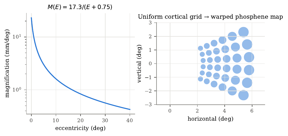
Figure 8. Retinotopy and cortical magnification. Left, the magnification function \(M(E) = 17.3/(E + 0.75)\) mm per degree on a logarithmic axis. Right, a uniform 6 by 6 electrode grid at 2.5 mm pitch placed along the cortical axis of the log map, mapped back to the visual field by the inverse map. Phosphene centers span about 2.4 to 5.8 degrees eccentricity with geometrically growing spacing, each drawn with diameter proportional to the inverse of magnification. The placement and size rule are illustrative; measured phosphene maps are less regular.

Why simultaneous stimulation blurs follows from superposition. In a resistive medium the potentials of simultaneous sources add, so two sources a distance \(s\) apart activate the midpoint when \(s \le 4r^*\), against \(s \le 2r^*\) when pulsed at different moments, so simultaneity doubles the separation at which two regions fuse. Interleaving removes this, which is how continuous interleaved sampling works. Current steering turns the same summation to advantage. Two sources driven together look to distant neurons like a single virtual electrode at the current-weighted centroid \(\bm{r}_{c} = (I_{1}\bm{r}_{1} + I_{2}\bm{r}_{2})/(I_{1} + I_{2})\), and changing the ratio slides it between them.

Dobelle and Mladejovsky (1974) stimulated the occipital cortex of awake patients through surface electrodes and catalogued the phenomenology. Usable phosphenes came only from primary visual cortex, at thresholds of 1 to 5 milliamps, electrode size mattered little, the map matched classical maps only roughly but was stable across sessions, two-point discrimination broke down between 2 and 3 mm, and phosphenes from several electrodes often blended. Each phosphene needed a train of five to fifteen pulses, which they turned into a design estimate of about 40 to 50 words per minute, and they estimated surgeons could place 50 to 200 electrodes per hemisphere at 3 mm centers over exposed striate cortex. Much of their quantitative detail came from one patient who gave about as much time as all the others combined, the study reported no statistics, and its milliamp currents through millimeter-scale discs may not transfer to microelectrodes. Beauchamp and colleagues (2020) showed that tracing a shape sequentially produces recognizable form vision. Designing letter sequences from each participant’s own phosphene map and stimulating electrodes one after another, with current steering to create virtual electrodes between contacts, they had a blind participant with a 60-electrode cortical implant identify forms with 90% of drawings in the correct cluster and verbal identification correct on 37 of 40 trials (chance 25%), and discriminate two forms at up to 86 per minute. Static stimulation never produced a recognizable letter. Current steering moved a phosphene predictably. Stimulating two Orion electrodes together, with each at a fraction of its own threshold current, produced phosphenes at intermediate positions along the line between their single-electrode locations, and the centroid model predicts the ordering to within the scatter of single reports. The main limit is scale. Five people, small alphabets of two to seven forms fitted to each person’s map, chance running from 14% to 50%, and some discriminations solvable from temporal order alone, since “up” and “down” use the same four electrodes in opposite orders. That a blind participant could still recognize forms from phosphenes two seconds apart suggests the benefit of sequencing extends beyond apparent motion.

On the auditory side, the cochlea maps frequency to place by the Greenwood function \(F(x) = A(10^{\alpha x} - k)\), whose inverse has the same log-plus-constant structure as the visual map, so a uniform array samples both stimulus spaces in roughly constant proportional steps. Continuous interleaved sampling (CIS) splits sound into bands, extracts each band’s slow envelope by rectification and low-pass filtering (the rectified cosine’s harmonics all sit at twice the carrier or higher, so the filter leaves only the envelope), compresses it logarithmically into the narrow range electric hearing tolerates, and modulates interleaved pulse trains offset in time, so each field acts alone.

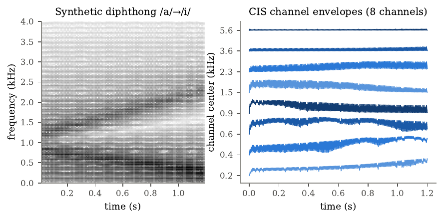
Figure 9. Continuous interleaved sampling on a synthetic diphthong. Left, the spectrogram of a 120 Hz pulse train passed through two time-varying resonators approximating the glide from /a/ to /i/, with the first formant falling and the second rising. Right, the envelopes of eight CIS channels from log-spaced bandpass filters, rectification, a 200 Hz low-pass filter, and logarithmic compression. The formant motion appears as energy shifting across channels, so CIS conveys spectral shape as a moving pattern across a few broad channels without any explicit formant tracking.

The cochlear implant has a long prehistory, from Volta’s battery across the ears around 1800 to the first multichannel implants in Vienna and Melbourne in the late 1970s and the Nucleus device’s FDA approval in 1985, with recipients growing from a few thousand in 1988 to about one million by 2022. Speech in quiet needs only a handful of envelope channels, since normal-hearing listeners understand speech in simple sentences from the envelopes of just three or four noise bands, and CI users improve with electrode count only up to about seven or eight because fields from neighboring electrodes overlap in the conductive fluid and the electrodes sit far from the spiral ganglion. So eight channels meet two facts at once. Zeng’s 2022 perspective on the millionth cochlear implant argues that multichannel envelope processing raised average sentence recognition in quiet to 70 to 80%, but that average performance has held flat for about 30 years. In Zeng’s account the plateau is this long, and he pins it on the electrode design, unchanged since its inception. His diagnosis is that the scala tympani electrode design, unchanged since its inception, is now the bottleneck, and that the imprecision of how current reaches the target neurons now outweighs any gain from better encoding. Zeng traces the history through three milestones in open-set sentence recognition. House’s single-channel device gave minimal open-set recognition, Clark’s multichannel Nucleus-22 reached about 30%, and Wilson’s CIS reached 70 to 80% in quiet, a jump produced by signal processing on the same kind of array. The earlier feature-extraction processors, which tried to place a formant at a precise cochlear location, broke down because electrode position varied with insertion, nerve survival varied between people, and current spread blurred the tonotopy, so a strategy that must hit an exact place breaks down under all of these. Envelope coding succeeded because intelligibility rests on slow modulation across a few broad bands, the carrier matters little, and interleaving removes the interaction of simultaneous fields. Zeng also uses the CI as a research tool. Electric loudness grows exponentially with current, implying a central transformation from compression to expansion, since if compression were entirely cochlear electric stimulation should give linear loudness growth.

The three papers share a map that is logarithmic with a linear core, and all three use time to separate what space leaves blurred, CIS at microseconds and sequential visual stimulation at tens to hundreds of milliseconds. Current steering traveled from the cochlea to the cortex; Zeng’s caution is that in CIs it created many more discriminable pitches while speech scores held flat, which is the test any visual version must pass. The two fields also measure success differently, the CI field with open-set sentence recognition in large populations and the visual field with forced choice among a handful of forms in a few people, so an open-set visual measure such as reading arbitrary words would make the two comparable. Monkey work with a thousand channels in V1 and V4 found animals recognizing static patterned stimulation as letters and motion, which complicates the claim that static stimulation cannot produce form and suggests the limit may hold only at the scale of surface electrodes, where activated patches are millimeters wide.

Restoring communication, speech and typing

Some people lose the ability to speak while the cortex that plans speech keeps working, from a brainstem stroke or from ALS. A communication BCI records the cortical activity of attempted speech or attempted hand movement and converts it to text or sound. The output is a discrete sequence arriving at a pace the user chooses, and the timing of each symbol goes unrecorded, so the decoder must read a sequence whose alignment to the neural data is unknown. Speech is a motor act, produced by shaping a sound source with a movable filter, so each sound corresponds to a configuration of the lips, tongue, jaw, velum, and larynx, and those articulators are represented in ventral sensorimotor cortex, below the hand along the precentral gyrus. Damage to the corticobulbar pathway, from a pontine stroke or from ALS, abolishes speech while leaving that cortex intact, which is why the commands persist after the pathway to the muscles fails. Both speech groups decode about 39 phonemes and spell words with a pronunciation dictionary, which frees the vocabulary from a rehearsed word list, so a decoder trained on about ten thousand sentences can output any of 125,000 words. Consonants differ in place of articulation, manner, and voicing, and because area 6v appears to represent phonemes by how they are made, decoders confuse phonemes produced in similar ways, a fact that recurs across all three studies.

Connectionist temporal classification (CTC) solves the alignment problem by treating it as a hidden variable. Adding a blank symbol and a collapse map \(\mathcal{B}\) that merges repeats then deletes blanks, the probability of a label sequence is the total probability of all paths that collapse to it,

\[P(\bm{y} \mid \bm{x}) = \sum_{\pi \in \mathcal{B}^{-1}(\bm{y})} \prod_{t=1}^T p_{t}(\pi_{t}),\]

which a forward dynamic program over an extended label sequence computes in time \(O(TU)\). The gradient against the network’s scores works out to \(p_{t}(k) - \gamma_{t}(k)\), where \(\gamma_{t}(k)\) is the posterior that a path spelling the target emits symbol \(k\) at step \(t\), so CTC training is frame-wise classification against soft labels that are the model’s own recomputed best guess at the alignment.

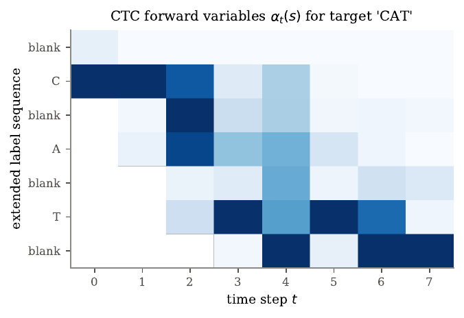
Figure 10. CTC forward variables for the target CAT on an eight-step toy example over the symbols blank, C, A, T. Rows are the seven positions of the extended label sequence (blank, C, blank, A, blank, T, blank), columns are time steps, and each column is normalized to its maximum for display. The lattice has a staircase shape, since a path cannot reach T before emitting C and A, and a path still on C cannot finish in time. The total is \(\log P(\mathrm{CAT}\mid\bm{x}) = -4.467\), and the companion code agrees with brute-force enumeration to machine precision.

CTC assumes the symbols in a path are conditionally independent given the input, which is weaker than it looks, since each step’s distribution comes from a recurrent network that has seen context, but the model treats each output as independent of the others, which is one reason a separate language model is added. An \(n\)-gram model assigns \(P(w_{i} \mid \text{history})\) from corpus counts, smoothed so that every \(n\)-gram keeps a nonzero probability, and the decoder maximizes a weighted objective \(\log P_{\mathrm{neural}} + \lambda\log P_{\mathrm{LM}} + \beta\vert W\vert\) with beam search, which keeps the best few partial hypotheses at each step and merges those that collapse to the same prefix. The word-insertion bonus \(\beta\) counteracts the tendency to drop words, since every word multiplies the language-model probability by a number below one. Willett and Jude compiled the collapse rule, a pronunciation lexicon, and the grammar into one weighted finite-state transducer, with each beam-search step taking under a millisecond, and used a larger neural language model to rescore the best candidates offline. Word error rate measures accuracy, the Levenshtein edit distance divided by the number of reference words, which can exceed 100% because insertions count, and which papers aggregate in at least three incompatible ways.

Willett and colleagues (2023) decoded attempted speech from four Utah arrays in areas 6v and 44 of a woman with ALS, using a five-layer gated-recurrent network trained with CTC and a trigram language model. Real-time decoding reached a 9.1% word error rate on a 50-word vocabulary and 23.8% on a 125,000-word vocabulary, the first successful large-vocabulary decoding, at 62 words per minute, more than tripling the handwriting BCI’s 18. Even eight years into dysarthria, area 6v still represented speech sounds by how they are made, which is what lets the decoder generalize to a 125,000-word vocabulary. Area 6v carried rich information (92% accuracy across 33 orofacial movements) while area 44 carried little. Saliency analysis showed the decoder confused phonemes articulated in similar ways, and the similarity structure matched articulator trajectories at 0.61, so eight years into dysarthria area 6v still represented speech sounds by how they are made. The authors note that 24% likely remains too high for everyday use, there was one participant who could still partly vocalize, and about 140 minutes of data collection and retraining preceded each day’s evaluation (omitting same-day data raised offline error to 30%). Metzger and colleagues (2023) decoded from a 253-electrode ECoG grid in a woman anarthric for 18 years, reaching a median of 78 words per minute and a 25% word error rate on a 1,024-word vocabulary, and extended decoding to synthesized speech and a controllable avatar, with facial animation decoded above chance and nine emotional expressions at 74%. (A 2024 correction reports a channel-ordering error that changed the anatomical analyses while leaving the decoding performance intact, so I make no anatomical claims from the uncorrected text.) A small 26-word-plus-finger classifier held 96.8% accuracy across 19 sessions under a fixed fit, even after a 61-day gap, which the authors contrast with the sentence decoder they trained on preceding days. Offline, expanding the vocabulary to 39,378 words left the word error rate statistically unchanged, and on the constrained augmentative-communication phrase sets the offline rates fell to 4.92% at 101 words per minute. Because the network was bidirectional and text appeared only after silence detection, “real time” here means sentence by sentence, and the 78 words per minute figure was measured with instructed pauses between words.

Jude and colleagues (2026) applied the same recipe to the hand, decoding a 30-key bimanual QWERTY keyboard from attempted finger movements (three movements per finger select the three keyboard rows). The participant with spinal cord injury, with 384 hand-area electrodes, typed with a word error rate below 7% in every block and a peak of 110 characters per minute, or 22 words per minute. Keyboard errors concentrated on the same or adjacent fingers and were easier for a language model to correct than handwriting errors at high error rates, which the authors turn into a design principle. All three systems share the recipe (a recurrent network with CTC plus a language model) and differ in almost everything else, and all three produce errors that follow motor similarity, so the errors reveal the geometry of the neural representation. All depend heavily on the language model, which has a cost. A model trained on common text can override unusual names or strings, which is why Jude’s system must turn its language model off for two-factor codes. Jude’s error structure supports a design principle. Since adjacent-key swaps often produce non-words the lexicon rejects, keyboard errors above a raw character error rate of about 25% were less likely than handwriting errors to survive into the output. The typing decoder also calibrated faster, reaching 7% word error with 30 sentences where a handwriting decoder needed 70, and kept more of its accuracy at low electrode counts, with a 9.5% word error at 140 electrodes against 27% for handwriting. At 22 words per minute typing is still well below the 62 to 78 of the speech systems, so its case rests on freedom from articulator control, privacy, and ease of language-model repair. A follow-up by Card and colleagues reported 90.2% accuracy on a 125,000-word vocabulary on the second day of use and about 32 words per minute in self-paced conversation over more than 248 hours, still well below natural conversation’s 160. Across all of this work the papers aggregate error rates in at least three incompatible ways and measure speed over different windows, and copy tasks dominate, so a shared benchmark that includes free conversation would let the systems be compared on equal terms.

Inner speech and mental privacy

The speech prostheses decode attempted speech, which is tiring and depends on breath control. A decoder that worked from speech the user only imagines would avoid those costs, but it raises a question new to attempted-speech devices. If the same cortex represents words a person says to themselves, a device built to decode intended speech might pick up words the person meant to keep private. Inner speech is silent speech directed to the self, and the review by Fernyhough and Borghi (2023) stresses that it varies in form, from full sentences to condensed fragments and from a single voice to a dialogue, that some people report little or none, and that inner speech produced on instruction may differ from the inner speech of ordinary thought. Every decoding study cues a known word and asks the participant to say it internally, so whether these decoders generalize to spontaneous inner speech is the empirical question on which the privacy debate turns.

Vygotsky’s developmental account, which Fernyhough and Borghi build on, holds that language first appears as social dialogue, becomes private speech spoken aloud to the self, and is then internalized as inner speech, abbreviating along the way, so inner speech is more than social speech with the movement removed. Two dimensions matter most for decoding. Inner speech can be expanded into full sentences or condensed into fragments, and monologic with one voice or dialogic between perspectives. Measuring a private experience is itself hard, since only the person producing it can observe it; questionnaires are easy to administer but report beliefs about one’s own mind, while descriptive experience sampling, which beeps at random moments and elicits a trained description, often diverges from them. People differ widely, some report almost no inner speech at all, and the review’s sharpest warning for decoding is that instructed inner speech may be some way removed from the inner speech of ordinary thought.

We can order speech modes by how much of the motor act they retain, from attempted vocalized speech through attempted mimed speech to motoric, first-person auditory, and third-person auditory inner speech. Decoding becomes harder along this continuum for several reasons. If inner speech scales the word-specific part of the response by \(\alpha < 1\), the Mahalanobis distance between words becomes \(\alpha\Delta\) and the two-class error rate becomes \(\Phi(-\alpha\Delta/2)\); since \(\Phi\) is steep near the origin, a word pair with error \(\Phi(-2) \approx 2.3\%\) under attempted speech jumps to \(\Phi(-1) \approx 15.9\%\) when the separation halves. Inner speech also leaves no motor output to verify compliance, no ground-truth timing, and a strategy that varies across participants and days. Cross-condition generalization tests whether codes are shared. Under a shared-but-scaled model \(\bm{\mu}_{k}^{\text{inner}} = \bm{c} + \alpha\bm{m}_{k}\), word patterns point the same way but are shorter, matching an activation-threshold account in which inner speech engages the same population while stopping short of movement; under an orthogonal model the word structure lies in directions separate from those attempted speech uses. A nearest-centroid decoder trained on attempted speech and shown an inner-speech trial favors the correct word through a signal term \(\alpha\bm{m}_{j}^\top(\bm{m}_{k} - \bm{m}_{l})\) that shrinks with \(\alpha\), so transfer is weaker than within-condition decoding, while a centroid offset biases it toward words aligned with the shift unless each condition is centered separately. Under the orthogonal model the signal term vanishes, so above-chance transfer from attempted to inner speech rules out strictly orthogonal codes.

Small-vocabulary claims need care about statistics. With \(K\) classes, chance is \(1/K\), but a finite test set fluctuates around it, so a binomial test sets the threshold. For seven classes at the 0.05 level, 70 trials need 16 correct (22.9%) but 280 trials need only 51 (18.2%). Trials within a session share slow fluctuations, so errors cluster in time and the binomial test is anti-conservative, and a Wilson or Clopper-Pearson interval, which stays within \([0,1]\) and keeps a nonzero width near 100%, is safer than the Wald interval. When \(n\) trials run clean, the rule of three bounds the failure rate at about \(3/n\), so 40 clean trials bound a rate only at 7.5%, and a rate below one in a thousand would need about 3,000 clean trials, a figure that matters for any privacy safeguard.

Wandelt and colleagues (2024) recorded single neurons from the supramarginal gyrus of two men with tetraplegia and decoded a set of eight cued words (six actual words, two pseudowords). The decoder read internal speech offline at 55% and online at 79% in participant P1 (chance 12.5%, best run 91%), and at 24% offline and 23% online in P2. A control array in hand-and-arm S1 modulated only during vocalized speech and stayed at chance for words, arguing against gross movement. Internal and vocalized speech shared many tuned neurons (82 to 85% overlap) while remaining distinct, so the authors recommend training decoders on internal speech directly. Kunz and colleagues (2025) recorded multiunit activity from speech motor cortex in four participants and found inner speech, listening, and silent reading all represented in the precentral gyrus. Inner speech resembled a weaker, scaled-down version of attempted speech, with word distances about 52% of those for attempted speech, supporting a shared-subspace over an orthogonal account. Real-time inner-speech sentence decoding reached word error rates of 14 to 33% on a 50-word vocabulary. The key privacy finding was that a decoder trained only on attempted speech decoded inner speech above chance in all three participants tested, so an attempted-speech BCI built the usual way could produce output during inner speech. This is the result in the whole guide with the heaviest implications, since the leak falls out of the ordinary way one builds a decoder, long before anyone sets out to read private thought. In constrained tasks, fragments of uninstructed inner speech reached the decoder. In serial recall the decoder read all three positions of a rehearsed sequence, and in counting the decoded numbers rose with position. The serial-recall and counting results used a number-only language model and binary pairwise classification, both far weaker than open-vocabulary decoding, and are the first tests of inner speech participants produced for their own purposes rather than on instruction. After verbal prompts such as recalling song lyrics the decoder emitted more words than after a clear-your-mind instruction, 22.3 against 5.8 for one participant, but the output was mostly gibberish with occasional plausible phrases, and the authors deliberately withheld the decoded text and stopped short of decoding intelligible free-form thought. The gap between instructed and spontaneous inner speech remains large, which is both the scientific basis for the privacy concern and the reason its current reach is limited.

Kunz and colleagues then showed that the shared code is offset along a “motor-intent dimension,” the axis \(\bm{u}\) separating inner from attempted speech, present even in the anarthric participant. Projecting that axis out left word decoding intact while sharply reducing the ability to tell attempting from imagining, which gives two safeguards. Imagery-silenced training adds inner-speech sentences to an attempted-speech decoder labeled with the silence token, so it learns to emit the silence token for inner speech. A keyword gate keeps an inner-speech decoder silent until it detects an imagined keyword; in one session it was correct on 98.75% of 80 cued trials, though the false-opening rate during hours of spontaneous thought, the quantity that matters, remains unmeasured. Proposals for neurorights are ethical arguments, while Chile’s constitutional amendment protecting brain activity and Colorado’s addition of neural data to sensitive categories are law, and how either law applies to an implanted research device stays unsettled in my sources. The decoding results establish facts (an attempted-speech decoder responds to inner speech, some uninstructed inner speech is detectable, free-form thought was not decoded); the claim that existing protections are inadequate is a separate argument, one that needs more than the results alone. Technical safeguards govern what leaves the decoder, while recording and storage lie outside their reach, so a device could suppress inner-speech output while storing recordings a better future model might decode, which makes technical and legal protections complementary. The two decoding studies agree on their central finding while differing in almost every design choice. Wandelt recorded single neurons in parietal cortex of people who could speak, Kunz recorded multiunit activity in motor cortex of people with impaired speech and decoded sentences as well as words. “Similar but distinct” and “a scaled-down version offset along a motor-intent axis” are compatible descriptions, since a scaled, offset code produces the partial cross-decoding and partial neuron overlap that both report. Variability across participants was high, which array placement explains in part, and the review suggests another source. If a person’s inner speech lies near the motor pole of the simulation-to-abstraction continuum, a motor-cortex decoder will work better for them, a hypothesis no study has yet tested by pairing recordings with an independent measure of inner-speech phenomenology.

Closing the loop on mood, neuromodulation for psychiatry

Psychiatric neuromodulation writes into the brain to change a mood, and the only readout here is a clinical rating made days or weeks later by a person who knows they have had brain surgery. This shapes the whole field. The target signal is slow, sparse, and subjective, and the evidence is unusually vulnerable to bias, because people enroll at their worst and people at their worst tend to improve whatever is done. Deep brain stimulation (DBS) delivers chronic high-frequency pulses through implanted leads, borrowed from Parkinson’s disease, where high-frequency stimulation of overactive circuits improves symptoms. Its mechanism remains unsettled even for movement disorders. Stimulation can silence local cell bodies while driving output along passing axons, or replace a pathological activity pattern with a regular low-information one, or change activity across a whole circuit through activated projections. Mayberg’s team framed the subgenual cingulate target in terms of silencing an overactive region, but placed the electrodes in the adjacent white matter, which activates passing fibers and is closer to the network account, and the later move to tractography-guided targeting follows from that second reading. In an open-label study without a control, improvement combines the treatment effect with placebo, natural course, and regression to the mean. If two severity scores are jointly normal with correlation \(\rho\), then \(\mathbb{E}[X_{2} \mid X_{1}] = \mu + \rho(X_{1} - \mu)\), so a patient scoring high at baseline is expected to improve by \((1-\rho)\) times their excess even untreated. Enrolling only patients above a threshold \(c\) makes this systematic, since the enrolled cohort’s expected untreated improvement is \((1-\rho)\sigma\lambda(\alpha)\) with \(\lambda\) the inverse Mills ratio, growing as the correlation falls and the threshold rises. A randomized sham-controlled trial subtracts all of these at once, because the sham group undergoes the same surgery, threshold, and expectations, so they cancel in the difference, but it needs many more participants, each of whom undergoes neurosurgery.

Mayberg and colleagues (2005) reported the first six patients with treatment-resistant depression to receive DBS of the white matter next to the subgenual cingulate (area 25). All six reported acute effects time-locked to stimulation at specific contacts and absent with sham, described as “sudden calmness or lightness.” Over six months, group mean depression score fell from 25.8 to 11.5, and four of six met the response criterion. The paper’s Summary reports “remission of depression in four of six patients,” but applying the paper’s own definitions to its own six-month scores gives response in four and remission in two, since only two patients fell below the remission threshold of 8. I worked the paper’s own definitions back through its own scores, and a reader taking the Summary at face value doubles the remission rate. The strongest evidence that stimulation itself mattered was a single blinded discontinuation in the best responder, whose mood declined over weeks off stimulation and normalized within about 48 hours of a blinded restart. There was no control group, and the later multisite randomized sham-controlled BROADEN trial found 20% responders with active stimulation against 17% with sham, a non-significant difference, and stopped for futility. Applying the standard error of a difference in proportions to the BROADEN counts gives a 95% interval from about -0.13 to 0.20, consistent with no effect and ruling out the large open-label-versus-sham gaps, while still allowing a moderate benefit or a subgroup effect. Later open-label work with tractography targeting and with LFP sensing reported high response rates again, which must be read against that 17% sham rate.

Oganesian and Shanechi (2024) take the failure of fixed stimulation as a starting point and propose closed-loop, personalized neuromodulation. A closed-loop system needs an estimate of a hidden mood state, which a state-space model supplies by combining continuous neural features with sparse ratings. The Kalman filter handles the sparse labels directly. A missing rating is a rating with infinite noise variance, which drives its column of the gain to zero, so the filter uses every rating when one exists and runs on neural features in between, decoding mood as \(\bm{T}\hat{\bm{x}}_{k}\). Given the state, a controller decides the stimulation. Proportional control leaves a steady offset when a constant drift pushes the system away from target, because holding the state against the drift needs constant stimulation and a proportional controller can deliver that only through a constant error; adding integral control removes the offset, since at equilibrium the accumulated error must be constant, forcing it to zero. Delay is the harder problem. For proportional control with a delay of \(D\) steps, the characteristic equation \(z^{D+1} - az^D + bk_{p} = 0\) has a shrinking stable range, so a slow, delayed biomarker forces a gentle, slow controller. Model-based control needs the matrix saying how stimulation moves the state, which requires system identification with a persistently exciting input, since stimulation held at a fixed setting confounds its own effect with the drift.

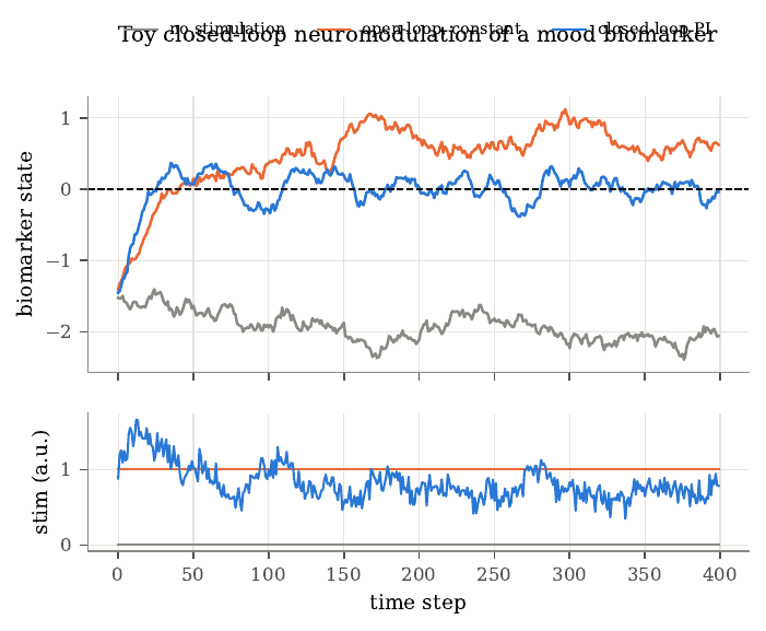
Figure 11. Toy closed-loop neuromodulation of an invented biomarker. Top, the biomarker state under a linear model that drifts toward a negative value; the dashed line marks the target. Without stimulation the state settles near -2, constant open-loop stimulation overshoots and settles near 0.67, and a proportional-integral controller acting on a noisy, five-step-delayed measurement holds the state near the target. Bottom, the stimulation delivered by each strategy. The model is a toy with no claim about actual mood dynamics; it illustrates why a fixed dose is right only for a fixed patient, and why delay forces a gentle controller.

The review establishes, by synthesis, that open-loop DBS for depression has fallen short in controlled trials, that candidate biomarkers are heterogeneous and rest on cohorts of fewer than about 13 people, and that clinical closed-loop work has so far used simple on-off triggering. It proposes that model-based closed-loop control would do better, a proposal it does not yet establish, and it writes from within one research program whose senior author holds patents on the proposed methods. The closed-loop program inherits Mayberg’s inferential problem in a new form, since biomarkers chosen by correlating many neural features with a few dozen ratings in small groups will look worse on new data, a selection effect related to regression to the mean. Validation on held-out time periods and patients, and eventually randomized comparisons, is the closed-loop analogue of the sham-controlled trial.

The timescales make the control problem unusually hard. In Mayberg’s series sleep changed in the first week, response accumulated over one to two months, and in the single discontinuation symptoms returned over weeks and resolved within about 48 hours of restart. A controller that regulates a fast neural feature may be stable while leaving mood untouched, and one that regulates mood directly must be slow. The biomarker is also noisy, because neural features relate to mood weakly, and the labels are sparse, because ratings come a few times a day. The review surveys candidate biomarkers, mostly spectral power and coherence in orbitofrontal, amygdala, and cingulate regions for depression, all from cohorts of fewer than about 13 people, and reports that the first closed-loop depression case used an amygdala gamma-power biomarker to trigger on-off stimulation in one patient. Current sensing-capable devices have only four or eight contacts per lead and can run only simple on-device algorithms such as linear discriminant analysis, so the multiregional continuously learning decoder the review proposes would exceed what today’s hardware allows. Identifying a dose-response also requires persistently exciting stimulation, built from noise-modulated pulse trains, and every period of exploratory stimulation keeps a severely ill patient off the best known setting, which turns the familiar exploration-exploitation tradeoff into an ethical one.

Ultrasound, a new window onto the brain

Every recording method trades how much of the brain it sees against how finely it resolves what it sees. Functional ultrasound (fUS) takes a distinctive position. It images changes in local blood volume across a plane several centimeters wide and deep, at a resolution near 100 micrometers, from outside the dura. The price is the skull, because bone absorbs and distorts sound at the frequencies needed for fine imaging. Wavelength is \(\lambda = c/f\), about 99 micrometers for the 15.6 MHz macaque probe and 205 micrometers for the 7.5 MHz human probe, and these track the stated resolutions. Attenuation grows with frequency, \(L(z, f) = 2\alpha_{0} f z\) decibels, so for a fixed loss budget frequency times penetration depth is roughly constant, and halving the wavelength halves the reachable depth. Bone attenuates far more than soft tissue and distorts the wavefront, which is why imaging at 5 to 18 MHz has needed an opening in the skull while neuromodulation near 500 kHz can cross it. Bone also reflects, because its acoustic impedance \(Z = \rho c\) is several times that of tissue, and it aberrates, because sound travels about twice as fast in bone, so a half-millimeter thickness variation across the probe shifts parts of the wavefront by more than a cycle at 7.5 MHz but less than a tenth of a cycle at 500 kHz, which is why the imaging and stimulation regimes diverge. Pulse-echo imaging maps echo arrival time onto depth, \(z = ct/2\), and resolution follows the pulse. Axial resolution is about half the pulse length, \(\Delta z \approx c/(2B)\) for bandwidth \(B\), and lateral resolution is the diffraction-limited spot \(\Delta x \approx \lambda z / A\) for aperture \(A\), which for the macaque probe gives about 100 micrometers, matching its reported value. A fixed lens sets the slice thickness perpendicular to the plane, so each pixel averages over a slab several times thicker than its in-plane size.

Ultrafast imaging insonifies the whole field with each tilted plane-wave transmission and forms every pixel by delay-and-sum beamforming, reaching thousands of frames per second. Coherent compounding sums beamformed images from several tilt angles to synthesize a transmit focus after the fact, since echoes from a point add in phase across angles while leakage carries angle-dependent phases and cancels. The Doppler shift of moving blood is \(f_{D} = 2f_{0} v\cos\theta/c\), tens to a few hundred hertz for brain blood flow, and power Doppler averages the squared blood signal over an ensemble,

\[\mathrm{PD}(\bm{x}) = \frac{1}{N}\sum_{t=1}^N \vert s_{b}(\bm{x}, t)\vert ^2,\]

which tracks blood volume, because the expected power of \(K\) independently phased red cells is \(K\,\mathbb{E}[a^2]\), proportional to the number of moving scatterers. Power tolerates aliasing, since folding a Doppler frequency preserves the signal’s energy.

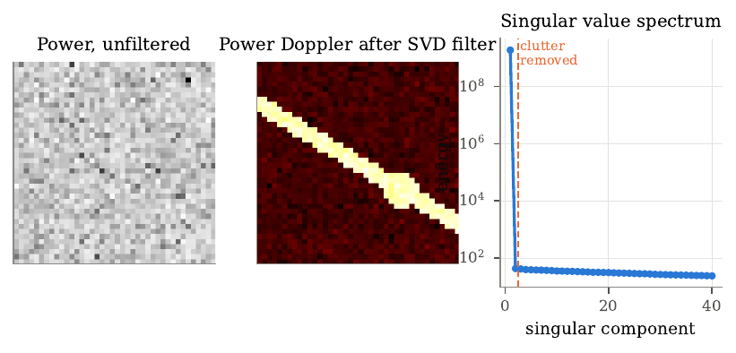
Figure 12. Simulated SVD clutter filtering. Left, the mean power of a raw ensemble (40 by 40 pixels, 200 frames), in which spatially coherent slow tissue clutter dominates and the vessels are invisible, with a vessel-to-background ratio of 0.91. Center, power Doppler after removing the first two singular components of the space-by-time Casorati matrix; the vessels, carrying a weak higher-Doppler blood signal, appear with a ratio of 9.9. Right, the squared singular values, with the first component holding nearly all the energy and the rest a low, nearly flat spectrum shared by blood and noise. Tissue echoes exceed blood echoes by orders of magnitude, so a plain high-pass filter fails when slow flow and tissue motion overlap in frequency; SVD filtering uses spatial coherence instead, since tissue moves coherently and so occupies a few leading components of the matrix.

Functional ultrasound reads activity through neurovascular coupling, a low-pass filter with a delay of seconds, so the hemodynamic response caps how fast an ultrasound BCI can respond, however fast the scanner runs. This favors decoding goals that persist, such as a held movement plan. A latency budget makes the limit concrete. In the macaque system each image integrates 0.4 seconds, about 800 milliseconds pass from the end of the pulse sequence to the formed image, and the task link adds a 31-millisecond round trip, so the newest data in a decision are at least about 0.83 seconds old, and the neural events behind them occurred seconds earlier through the hemodynamic response. Intracortical BCIs decode spikes in bins of tens of milliseconds, so faster ultrasound hardware alone leaves this gap open. The decoder reduces each high-dimensional image with principal component analysis, needed because the pooled within-class covariance from a few hundred trials is singular for tens of thousands of pixels, and classifies with linear discriminant analysis, which here uses the full covariance because neighboring pixels correlate strongly. Because blood vessels stay where they are, decoders can be carried across sessions by registering the anatomical vascular image with a rigid transform, in place of aligning neural statistics as the Degenhart stabilizer does; Degenhart aligned population structure because the neurons under each electrode change, while Griggs aligned anatomy because the vessels stay put, which runs on anatomy alone. Griggs and colleagues (2024) drove a closed-loop BCI in two macaques, decoding memory-guided movement plans from posterior parietal cortex at 2 Hz through a craniectomy. The monkeys selected among two or eight directions, and pretraining on registered data from weeks earlier let a decoder reach significance within about ten trials in the better animal. For two directions the better monkey reached about 80% (chance 50%), and for eight directions a mean angular error of 38 degrees (guessing gives 90). The most informative saccade voxels lay 5 to 9 mm below the surface, beyond the reach of surface or shallow penetrating arrays. The signal a decoder wanted sat several millimeters deep, where the less invasive electrode methods cannot see. The BCI makes one discrete choice per trial after a long delay, both animals were healthy, and many across-session numbers come from offline replays. Rabut and colleagues (2024) imaged a man’s brain through an acoustically transparent PMMA skull implant placed during a routine cranioplasty, while he played a video game and a guitar. Through a 2 mm window the cortical vasculature was visible, a general linear model found task-modulated regions, and a decoder classified task from rest at 84.7%, with most errors at block transitions from the hemodynamic lag. PMMA attenuated less than titanium mesh, and thinner was better. In rats, whole-brain Doppler intensity fell 35% under 1 mm of PMMA, 50% at 2 mm, 64% at 3 mm, and 66% under mesh, consistent with a reflection loss near 2 decibels plus a thickness-dependent absorption term, while titanium’s far higher impedance would reflect most of the sound. The participant had undergone a decompressive hemicraniectomy after a traumatic brain injury and received a custom PMMA cranioplasty with a thinned window, so the approach is minimally invasive only for patients who need cranioplasty anyway. This stops short of showing decoding of movement intention in a human, since rest and task differed in almost every respect, and the binomial significance test treats each 1.65-second image as independent when successive images within a block are strongly autocorrelated, so the effective number of trials is far smaller than the number of images. Together the two papers reduce the remaining gap to a human ultrasonic BCI to combining two demonstrated components, decoding and non-invasive access. Focused ultrasound is the natural write channel, and it is the only non-ionizing energy a device can focus in deep tissue, so at low frequencies it crosses the intact skull, at the cost of millimeter resolution. At high intensity it ablates tissue, and MRI-guided thalamotomy for essential tremor improved hand-tremor scores from 18.1 to 9.6 against a sham change of 16.0 to 15.8, which shows clinicians can focus sound onto deep targets precisely enough for therapy even if these are surgical treatments. At lower intensities, with circulating microbubbles, it transiently opens the blood-brain barrier, and at lower intensities still it modulates activity reversibly, with the leading hypothesis being mechanosensitive ion channels, though ultrasound can also vibrate the skull and activate the cochlea, so brain-wide responses that vanish after cutting the auditory nerves make sham controls essential. Imaging needs short wavelengths that bone attenuates over a round trip, while neuromodulation tolerates millimeter wavelengths on a one-way path, so a two-way interface could pair a high-frequency imaging probe behind a window with a low-frequency transducer on intact skull, separated in frequency or time to avoid interference. Building it requires a clearer account of how low-intensity ultrasound acts on neurons, with auditory confounds controlled, and a demonstration that imaging can detect the effects of stimulation in the same session. Both imaging papers also captured only one plane, most of which contributed little to decoding while informative tissue lay outside it, and volumetric functional ultrasound has reached a field of view of roughly 80 by 20 by 40 mm in humans, so the move from planes to volumes, which multiplies the data rate and the cost of the clutter filter, is the next step toward a usable human ultrasonic interface.

The chapters so far have read the field’s published work. This section turns to my own, where the measurement trade of the opening sections appears in a clinical decoding problem I have worked on directly, localizing an epileptic lesion from the recording, and asking what a second modality actually adds once you have it.

A worked case, localizing a lesion from EEG

To make the trade concrete, take the clinical question I know best. Can a recording of the brain’s electrical activity tell you where a lesion sits? Before epilepsy surgery, a workup has to point at the region to remove, and scalp EEG, together with the intracranial recordings a workup sometimes adds, is one of the signals clinicians read to find it. A focal lesion, like a small malformation of the cortex, can make a region fire abnormally, and the surgery with the best chance of seizure freedom removes that region. A model that could point at the region from the recording alone would be a usable clinical tool. The task I scored is a stripped-down version of it. Given a window of EEG, name the region, and compare the model against chance.

The hardest part here is chance. If you score the model as top-1 over a set of candidate regions, the naive chance level is one over the number of regions. Some regions carry a label far more often than others, so a model blind to the signal can still beat naive chance by guessing the common region. Getting that baseline right is most of the problem, and it is where my own first result went wrong.

Scoring localization as top-1 over 20 sensor pairs, against a density-matched chance baseline that already corrects for how many channels each window labels, my localizer scored 2.00 times chance. That is the number I first reported, and it reads like clear spatial skill. Then I ran a control for a different reason and it changed the reading. I pooled the model features across sensors, so the model keeps everything it learned and loses any access to which sensor is which, and scored that. A model with no spatial information should sit at chance. It sat well above. Pooled over one encoder it reached about 1.57 times chance, and over two others about 1.35 and 1.28, because it had learned which sensors are labeled most often. The density-matched baseline corrects for how many channels a window labels; the prior over which ones are likely slips through, and no amount of care in building it would have caught this. Against a model-free, prior-only predictor, the proper floor sits at about 1.37 times chance, well above 1.00.

So part of my 2.00 traced to a labeling prior, with the rest actual localization. The useful thing is that the signal survives once you denominate it correctly. Measured against the proper floor, the localizer still clears it by a margin, about 1.62 times the floor against the 2.00 times naive chance I first reported. There is spatial information in the recording. The headline just overstated how much, and the right baseline turned out to be most of the work. The lesson repeated at a coarser scale and in the other direction. At hemisphere level, where there is no label to exploit, the same model-free predictor scored 0.729 times chance, below chance, because committing to one hemisphere is worse than guessing once windows with multi-hemisphere labels are counted. A low-cardinality balanced metric was safe to divide by. The high-cardinality one was treacherous.

Having signal and having useful signal are two different things, so I asked the next question directly. How accurate does a localization prior have to be before conditioning a lesion detector on it beats using no prior at all? I swept prior quality from chance to a perfect oracle and measured where conditioning started to pay. With enough seeds, a prior that is 90 percent accurate matches the no-prior baseline, indistinguishable from it at p equal to 0.55, so break-even sits at or above 90 percent accuracy. The bar sits this high, and finding it there reframed the whole fusion question for me. My localizer does not clearly clear that bar. The spatial signal exists, and it is right at the threshold where it would start to help, not clearly past it.

Figure 1. Signal at the edge of useful. Left, localization scored as a multiple of density-matched chance. A model with no spatial information already reaches 1.37 times chance, a model that keeps its features and loses sensor identity reaches 1.57, and the full localizer reaches 2.00, so part of the headline is a label-frequency prior. Against the proper floor the localizer still clears it, by a corrected 1.62 times the floor. Right, how accurate a prior has to be before it helps a lesion detector. Break-even sits at or above 0.90, and the localizer does not clearly clear it, so the spatial signal is at the edge of useful rather than past it. At hemisphere level, where there is no label to exploit, the same model-free predictor scores 0.729 times chance, below chance.

That localization work is one half of a larger point. The EEG is spatially weak, and the MRI has its own blind spot. Focal cortical dysplasia is a surgically treatable cause of drug-resistant epilepsy, and its lesions are often small and low contrast. A trained 3D nnU-Net on T2-FLAIR detects 150 of 175 confirmed lesions, 85.7 percent, and misses 25 of them with no voxel above threshold anywhere in the lesion. A number like 85.7 percent reads as a strong detector. It is also a detector that misses precisely the cases a clinician most needs help with, because the obvious lesions were visible without a model. The blind spot follows what the modality can see.

This is the argument for multimodality in medicine. The information that would rescue those 25 cases exists, and it sits in a different stream. In epilepsy, that stream is the EEG and the clinical workup, which point at a brain region independently of the MRI. If the model could use where the seizure localizes, it could lower its threshold there and raise it elsewhere, so a faint lesion in the right place survives while noise elsewhere is suppressed.

In my meeting notes, I have a related observation about simplicity bias, which needs checking before publishing. The note is that gradient descent tends to favor easily separable low-frequency linear features, like background color and texture, over complex nonlinear causal structure. That tendency fits this blind spot, since a detector can succeed on obvious lesions and still miss the subtle ones.

To measure the best case, I gave the recovery step a perfect localization prior. Each case contributed its own confirmed lesion lobe, as a stand-in for what an EEG workup would indicate. Restricting a multi-peak search to that region recovers 14 of the 25 missed lesions, every recovery within the top four candidates, against null baselines of 1.4 and 4.0 recoveries at P less than 10 to the power of negative 4. Measured against the null baselines, the recovery was this large, since every one landed within the top four candidates. That is a large effect, and it says the ceiling is worth reaching. The second modality, if it were perfect, would recover more than half of the complete misses.

A perfect prior lies beyond what a clinician can obtain, because a deployable pipeline has to find the region first, and no EEG signal was processed anywhere in that experiment. The 14 of 25 is an oracle upper bound, a ceiling, and I report it that way every time it appears. The question is what a realistic, imperfect prior buys, and the localization work above is the answer to that part. Getting a correct prior from measured EEG is the piece that is still at the edge of its baseline.

Here is where multimodality has a cost. When I fuse a prior at the strength an actual EEG localizer could supply, the benefit collapses. A 90 percent accurate prior applied after segmentation is statistically indistinguishable from no prior at all, with a break-even near chance at p approximately 0.55, and forcing a hard fusion into the pipeline hurts. I ran the hard fusion and measured a loss. It loses about 0.36 Dice and degrades the majority of cases. The gap between the oracle ceiling and the realistic floor is the entire problem, and it is invisible to anyone who only reports the oracle number.

pause prior accuracy 90%, lesions recovered beyond baseline ~0

The reason sits in the fusion. The useful information has to survive the way it is combined. A prior that is right most of the time still points the search at the wrong region often enough to cancel its gains, and a hard fusion lets those wrong votes overwrite good image evidence. The modality carries signal, and the fusion throws it away.

In my meeting notes on Lampinen et al. 2023, I have a finding that speaks to this fusion point, and it needs checking before publishing. In that study, small multimodal models, FLAVA and BLIP, predicted human target-word distributions better than a massive text-only model, text-only GPT-4, in a Visual World Paradigm with 600 human subjects tracking gaze on paused video clips. In my notes, BLIP layer 9 cross-attention, where text queries attend to visual key and value pairs, accounted for up to 70 percent of human gaze variance. Shuffling visual attention patches inverted gaze correlation, which my notes read as cross-modal binding over low-level saliency. Adding a modality helps when the binding holds and is tested by a control that breaks it. Hard fusion that lets one stream overwrite the other is the opposite of that kind of binding.

Two further pieces of this work say the same thing from different angles, and both are about measuring the decision rather than the score. First, when a localizer must decide whether to commit to an answer per patient, the signal that knows when it is right is cross-segment self-agreement. Routing on it, how often separate EEG segments point to the same hemisphere, answers patients at 90.3 percent accuracy at 37 percent coverage, against 72.9 percent for the best confidence gate at matched coverage. I measured both gates at matched coverage, and cross-segment agreement beat the confidence score the field usually trusts by this margin. The model already contains a better reliability signal than the one everyone reads off it. Second, a catalogue of seven corrections to my own EEG-localization work shows how easily a correctly computed multimodal number supports a wrong conclusion, from a chance baseline that flatters every model to a single-site result mistaken for a cohort-wide one.

In my meeting notes, I have a related caution called the behavioral alignment fallacy, which needs checking before publishing. The note is that identical outward behavior can rest on radically different internal strategies. That is why I focus on the decision and the reliability signal, beyond the score alone.

So where does reading the brain leave us?

In the same place medicine already is, necessary and hard. The method you choose to read the brain fixes a point on the space-time-invasiveness trade, and whatever that method gives up stays lost to a model downstream. That is why EEG localization is hard and why its margin over the right baseline is modest. It is also why a clinical decision needs more than one stream, and the focal-cortical-dysplasia blind spot proves a model has to reach for another modality the way a clinician does. But adding EEG to the MRI model states a hypothesis, and the result still has to be earned. The oracle ceiling says the prize is there, more than half of the complete misses are recoverable with a perfect prior. The realistic floor says the work is in the fusion. A second modality earns its place only when it adds information at the operating point where the decision is made, under a fusion that protects the first modality from its errors, and measured against the realistic accuracy it will actually have. Progress in reading the brain is movement along a trade that different applications resolve differently, and a clear statement of the baseline the next version has to beat.

Limitations

The recovery result is an oracle upper bound on a 175-case confirmed-FCD cohort, with the zone simulated from the confirmed lesion lobe in place of a measured EEG report, and the recovery step has no external test set yet. The EEG localizer baselines and the break-even and hard-fusion results are from the companion analyses and are specific to those pipelines and cohort definitions. A separate journal framing runs the same work on a larger all-comers cohort with different denominators, and the two must be kept apart. The routing result is an offline replay of a policy. I have not observed it in a clinician-and-model team.

Acknowledgements

This draws on the CortSeer and CLERA line of work, including the structural-functional FCD detection study and the evaluation check titled Right Number, Wrong Conclusion. Both are collaborative, and the venues, collaborators, and paper links are on my clinical machine learning project page.

My own results sharpen the field-wide picture, so I close with the problems the whole reading list leaves open.

Open problems and where the field is heading

Read together, the papers suggest several problems that cut across the whole guide. The clearest pattern is that reading is ahead of writing. Decoders recover attempted speech at 62 to 78 words per minute and finger movements precisely enough to fly a quadcopter, while stimulation still produces percepts described as useful but unnatural. The asymmetry has a physical basis. A recording electrode listens passively to nearby neurons and exploits the redundancy of a population, while a stimulating electrode drives every excitable element in its field, including passing axons, and must create a redundant pattern from outside with far fewer channels than the neurons it needs to drive. Two directions help, using decoders to search for the stimulation pattern whose evoked activity best matches a natural one, and relying on long-term learning, as the cochlear implant did with a crude signal.

A principled method for telling a clinical team which region to implant for a given person and goal is still missing, and a systematic within-participant comparison is rare because each implant carries cost and risk. In several sections the same idea recurred, that populations are more informative and more stable than single neurons, that representational geometry and low-dimensional manifolds persist even as recorded neurons change, and that BCI engineering is moving toward estimating a latent state and decoding from it. A natural next step is to pretrain decoders across people and adapt them to a new person with little data, which depends on whether neural latent spaces are similar enough across people, an open empirical question that Guan’s able-bodied-like finger geometry makes promising. Most human studies report one or two participants, which shows feasibility, leaving typical performance open, and the history of DBS for depression is a cautionary example of how small open-label studies mislead. Another recurring target is the somato-cognitive action network. If regions interleaved with the classic effector areas carry signals about whole-body action planning, posture, and physiological control, they may be decoding targets that straddle motor and cognitive roles, and depth recordings already suggest the superior node responds to several effectors, but whether its neurons carry information a BCI can use, or whether existing hand-knob arrays sit in a node of it, remains unshown. Privacy, agency, and access are the ethical counterparts of these technical questions. A device that decodes attempted speech acts on a deliberate act of communication, while one that could decode inner speech acts on something closer to thought, so it needs both technical safeguards such as decoding only when the user explicitly starts it and legal safeguards such as treating neural data as sensitive. When a decoder combines neural evidence with a language model, part of the output reflects the model’s expectations rather than the user’s intent, and a user who struggles to correct errors may come to accept words the model chose, so interfaces should show what was produced and make correction easy, and evaluation should measure how often the output differs from what the user meant, which often diverges from a word error rate against a cued sentence. Access may be the hardest problem. The devices here are expensive, need specialized surgical teams, and depend on continued support from the companies that built them, and the collapse of a commercial retinal implant, against the cochlear implant’s roughly one million users, shows that planning for long-term support and equitable access should begin while BCIs are still in trials. Most BCIs in this guide close a loop through the user, who sees or feels the output and adjusts, and several added a second loop through the device, from Taylor’s coadaptive updates to Degenhart’s stabilizer to closed-loop neuromodulation. Two loops that adapt at once can interfere, each chasing a moving target, and the field has yet to settle on a general account of when coadaptation converges and when it oscillates, a question that psychiatric applications sharpen because mood fluctuates over hours to weeks and a wrong adjustment may not show for days. The modalities themselves form a ladder of invasiveness, from scalp EEG through functional ultrasound, endovascular electrodes, and surface grids to penetrating arrays, and the field has tended to read it as one trade between signal quality and risk. The papers give a more detailed picture. The coarse endovascular signal supported home use with minimal recalibration, surface ECoG supported high-performance speech, and ultrasound decoded intentions from a slow signal over a large volume, so the right choice depends on whether the application needs a few reliable commands or the fastest available decoding. Matching modality to need, with careful estimates of benefit and risk, is as much a clinical and ethical problem as an engineering one. A future version of this reading list would add within-participant comparisons of targets, multi-participant trials with standard outcomes, stimulation patterns derived from models of natural activity, decoders pretrained across people, long-term home-use studies of how people actually use their devices, and work on the governance of neural data. The field’s task for the next decade is to turn demonstrations of what is possible into devices that work reliably, for many people, for many years.

Key references

• Penfield, W. and Boldrey, E. (1937). Somatic motor and sensory representation in the cerebral cortex of man as studied by electrical stimulation. Brain.
• Mountcastle, V. B. (1997). The columnar organization of the neocortex. Brain.
• Georgopoulos, A. P., Schwartz, A. B. and Kettner, R. E. (1986). Neuronal population coding of movement direction. Science.
• Tye, K. M., Miller, E. K., Taschbach, F. H., Benna, M. K., Rigotti, M. and Fusi, S. (2024). Mixed selectivity: cellular computations for complexity. Neuron.
• Willett, F. R., Deo, D. R., Avansino, D. T., Rezaii, P., Hochberg, L. R., Henderson, J. M. and Shenoy, K. V. (2020). Hand knob area of premotor cortex represents the whole body in a compositional way. Cell.
• Gordon, E. M., Chauvin, R. J., Van, A. N., et al. (2023). A somato-cognitive action network alternates with effector regions in motor cortex. Nature.
• Chivukula, S., Aflalo, T., Zhang, C., Rosario, E. R., Bari, A., Pouratian, N. and Andersen, R. A. (2025). Population encoding of observed and actual somatosensations in the human posterior parietal cortex. PNAS.
• Taylor, D. M., Helms Tillery, S. I. and Schwartz, A. B. (2002). Direct cortical control of 3D neuroprosthetic devices. Science.
• Hochberg, L. R., Serruya, M. D., Friehs, G. M., et al. (2006). Neuronal ensemble control of prosthetic devices by a human with tetraplegia. Nature.
• Wu, W., Gao, Y., Bienenstock, E., Donoghue, J. P. and Black, M. J. (2006). Bayesian population decoding of motor cortical activity using a Kalman filter. Neural Computation.
• Kalman, R. E. (1960). A new approach to linear filtering and prediction problems. Journal of Basic Engineering.
• Gilja, V., Nuyujukian, P., Chestek, C. A., et al. (2012). A high-performance neural prosthesis enabled by control algorithm design. Nature Neuroscience.
• Willsey, M. S., Shah, N. P., Avansino, D. T., et al. (2025). A high-performance brain-computer interface for finger decoding and quadcopter game control in an individual with paralysis. Nature Medicine.
• Aflalo, T., Kellis, S., Klaes, C., et al. (2015). Decoding motor imagery from the posterior parietal cortex of a tetraplegic human. Science.
• Schalk, G. (2008). Brain-computer symbiosis. Journal of Neural Engineering.
• Oxley, T. J., Yoo, P. E., Rind, G. S., et al. (2020). Motor neuroprosthesis implanted with neurointerventional surgery improves capacity for activities of daily living tasks in severe paralysis. Journal of NeuroInterventional Surgery.
• Pons, T. P., Garraghty, P. E., Ommaya, A. K., Kaas, J. H., Taub, E. and Mishkin, M. (1991). Massive cortical reorganization after sensory deafferentation in adult macaques. Science.
• Guan, C., Aflalo, T., Zhang, C. Y., et al. (2022). Stability of motor representations after paralysis. eLife.
• Degenhart, A. D., Bishop, W. E., Oby, E. R., et al. (2020). Stabilization of a brain-computer interface via the alignment of low-dimensional spaces of neural activity. Nature Biomedical Engineering.
• Pandarinath, C., O’Shea, D. J., Collins, J., et al. (2018). Inferring single-trial neural population dynamics using sequential auto-encoders. Nature Methods.
• Churchland, M. M., Cunningham, J. P., Kaufman, M. T., et al. (2012). Neural population dynamics during reaching. Nature.
• Kingma, D. P. and Welling, M. (2014). Auto-encoding variational Bayes. International Conference on Learning Representations.
• Flesher, S. N., Downey, J. E., Weiss, J. M., et al. (2021). A brain-computer interface that evokes tactile sensations improves robotic arm control. Science.
• Valle, G., Alamri, A. H., Downey, J. E., et al. (2025). Tactile edges and motion via patterned microstimulation of the human somatosensory cortex. Science.
• Dobelle, W. H. and Mladejovsky, M. G. (1974). Phosphenes produced by electrical stimulation of human occipital cortex, and their application to the development of a prosthesis for the blind. The Journal of Physiology.
• Beauchamp, M. S., Oswalt, D., Sun, P., et al. (2020). Dynamic stimulation of visual cortex produces form vision in sighted and blind humans. Cell.
• Zeng, F.-G. (2022). Celebrating the one millionth cochlear implant. JASA Express Letters.
• Schwartz, E. L. (1980). Computational anatomy and functional architecture of striate cortex. Vision Research.
• Graves, A., Fernández, S., Gomez, F. and Schmidhuber, J. (2006). Connectionist temporal classification: labelling unsegmented sequence data with recurrent neural networks. ICML.
• Willett, F. R., Kunz, E. M., Fan, C., et al. (2023). A high-performance speech neuroprosthesis. Nature.
• Metzger, S. L., Littlejohn, K. T., Silva, A. B., et al. (2023). A high-performance neuroprosthesis for speech decoding and avatar control. Nature.
• Jude, J. J., Levi-Aharoni, H., Acosta, A. J., et al. (2026). Restoring rapid natural bimanual typing with a neuroprosthesis after paralysis. Nature Neuroscience.
• Card, N. S., Wairagkar, M., Iacobacci, C., et al. (2024). An accurate and rapidly calibrating speech neuroprosthesis. New England Journal of Medicine.
• Wandelt, S. K., Bjånes, D. A., Pejsa, K., Lee, B., Liu, C. and Andersen, R. A. (2024). Representation of internal speech by single neurons in human supramarginal gyrus. Nature Human Behaviour.
• Kunz, E. M., Abramovich Krasa, B., Kamdar, F., et al. (2025). Inner speech in motor cortex and implications for speech neuroprostheses. Cell.
• Fernyhough, C. and Borghi, A. M. (2023). Inner speech as language process and cognitive tool. Trends in Cognitive Sciences.
• Mayberg, H. S., Lozano, A. M., Voon, V., et al. (2005). Deep brain stimulation for treatment-resistant depression. Neuron.
• Holtzheimer, P. E., Husain, M. M., Lisanby, S. H., et al. (2017). Subcallosal cingulate deep brain stimulation for treatment-resistant depression: a multisite, randomised, sham-controlled trial. The Lancet Psychiatry.
• Oganesian, L. L. and Shanechi, M. M. (2024). Brain-computer interfaces for neuropsychiatric disorders. Nature Reviews Bioengineering.
• Griggs, W. S., Norman, S. L., Deffieux, T., et al. (2024). Decoding motor plans using a closed-loop ultrasonic brain-machine interface. Nature Neuroscience.
• Rabut, C., Norman, S. L., Griggs, W. S., et al. (2024). Functional ultrasound imaging of human brain activity through an acoustically transparent cranial window. Science Translational Medicine.
• Macé, E., Montaldo, G., Cohen, I., Baulac, M., Fink, M. and Tanter, M. (2011). Functional ultrasound imaging of the brain. Nature Methods.
• Demené, C., Deffieux, T., Pernot, M., et al. (2015). Spatiotemporal clutter filtering of ultrafast ultrasound data highly increases Doppler and fUltrasound sensitivity. IEEE Transactions on Medical Imaging.