← writing, Guide, Oct 12, 2026
We need to think outside the (black)box
An evaluation defined on outputs is gameable and incomplete. Reading the computation is the complement, and inside a protein language model the instrument turns out to be the hard part.
TL;DR. I have spent a while trying to break evaluations, and the same thing happens every time. A score looks healthy on a fixed dataset and stops meaning anything the moment a model or a search optimizes against it. A zero-shot protein score ranks below counting mutations. A benchmark correlation stops predicting which designs a campaign should keep. A verifier certifies a scorer that memorized the answers. A rule that skips the question still half-answers a safety benchmark. These share one structural fact. An evaluation defined on outputs is gameable and incomplete, because the output is a projection of what the model actually did. The complement is interpretability, reading the computation behind the emission. Interpretability is easy to overread too. A probe that hits AUC 0.94 collapses on held-out mechanisms, and inside a protein language model function stays causally accessible only at an interior depth I cannot pin down, where six of my twelve claims invert once I name the control. So the version I am left with is a white-box evaluation with its controls named first, and most of the work is in the instrument.
The pattern, scores break under use
Start with the mechanism that recurs across them, the winner’s curse. Write any score as the true quality plus an error term,
\[s = f^{*} + \varepsilon.\]On an average example the error is noise and a correlation looks fine. Now let a search keep the highest-scoring candidate out of many. The kept candidate is the one whose error happened to be most favorable, so the error of the selected item is the maximum of many draws, and
\[\mathbb{E}\!\left[\max_{i \le n}\varepsilon_i\right] \text{ grows with } n.\]The more you search, the more error dominates the score. A proxy that looks trustworthy in bulk becomes useless where it is used, at the top of the ranking.
This happens in practice. On 504 measured PET-hydrolase variants, a zero-shot ESM-2 650M score ranks activity at a within-study Spearman of 0.01, below a plain mutation count at 0.25. The expensive model is the weakest scorer on the task it is sold for. Reported benchmark correlation explains half the variance in top-10% selection value and only 16% at top-1%, so the number decays as selection sharpens. And when the evaluator becomes a component of an agent, it becomes an attack surface. A scorer that memorizes the measured outcomes clears a trust gate at AUROC 0.991 and adds nothing, because the gate scored it on data it had already seen.
The usual response is to patch the benchmark. Add harder examples, de-duplicate, re-weight. That helps a specific leak and misses the general problem. A safety benchmark makes the point cleanly. On a hazardous-knowledge multiple-choice set, a rule that skips the question and picks the longest of four options scores 46.5% against 25% chance, and a classifier trained on the answer text alone reaches 34.6%. Part of the score is an artifact of how the options were written, so a model’s number is an upper bound on what it knows until that artifact is subtracted, and a drop in the number under an intervention, on its own, is weak evidence that the intervention removed knowledge.
Every one of these failures lives at the output. The score reads a model’s emissions, the benchmark summarizes emissions over a corpus, the gate reads emitted outcomes. Each stops at the emission and passes over the computation behind it. That is the ceiling. An output-level evaluation reads a solved task and a shortcut to the same output as identical, and a shortcut is what an optimizer finds first.
The complement, read the computation
Interpretability is the move that steps off the output. It asks what internal structure produced the answer, and whether that structure is the thing you think it is. I have argued the skeptical half of this too, that interpretability evidence is easy to overread, and I still believe it. A linear probe that recovers a concept is weak evidence that the model uses that concept. In one case a probe reads a mutational process out of an embedding at an AUC of 0.94 on familiar processes and collapses to 0.775% on held-out ones, so it had memorized a fingerprint in place of a mechanism. Decodability is where an evaluation starts, with the rest still ahead.
This is also where several meeting-note cautions of mine belong, because they say the same thing at different levels, and the whole second half of this essay is an attempt to live by them. These cautions and the representational-geometry results that follow come from meeting notes I am still verifying against their sources, so I attribute them once here instead of re-flagging each one along the way. The first is the behavioral alignment fallacy. Identical outward behavior can rest on radically different internal strategies. Standard neuro-AI metrics can report high alignment from superficial correlations in place of shared computational principles. Output agreement leaves the internal strategy open. The second is simplicity bias. Gradient descent prioritizes easily separable low-frequency linear features, background color and texture, over complex nonlinear causal structure. If a brain and a network latch onto the same superficial feature, RSA scores high while the model misses deep causal structure. That is a false-positive RSA result, and it needs checking before publication.
The comparative lens behind the geometry has a precedent in biology. Kidney mechanisms became clear by comparing extremes, the desert kangaroo rat with an enlarged medulla against the freshwater beaver, an example from my notes. The same comparative idea now applies to neural activity, treated as point clouds in high-dimensional space with each neuron as an axis. Neurons lack a 1-to-1 correspondence across subjects or networks. Procrustes, rigid rotations, breaks down across unequal dimensions, for example 1,000 biological neurons against 10,000 artificial units. The field answers with three related tools. RSA measures pairwise distances between stimulus responses, with a first-level RDM and a second-level RDM correlation. CCA variants, SVCCA and PWCCA, align canonical directions. CKA measures angles via centered dot products.
Here is the equivalence that fixes the reach of geometry. Centered RSA equals linear CKA. Both equal average linear decoding accuracy over randomized white-noise tasks, so geometry equals decodability. A geometry match shows that the same information can be decoded. It leaves open whether the computation matches.
Two results push that gap all the way open. A 2020 study makes the divergence concrete. Identical CNNs on CIFAR-10, trained on the same schedule and sample order, diverged under different random seeds. Deep layers showed only 44% consistency across seeds. Category centroids held at about 88% agreement while the seeds scrambled exemplar-level arrangements within categories. Training objectives enforce category separation and leave internal organization loose, so behavior can match while geometry diverges. A 2026 eNeuro proof pushes further. Representation can be mathematically decoupled from causal computation. Two networks can run identical input-output computation with homomorphically encrypted geometries, giving an alignment score near zero. Enforcing geometric matching may impose unnecessary constraints if computation is substrate-independent. Geometry is one kind of evidence. It leaves open whether computation matches.
The skeptical half is an argument for doing interpretability carefully, and for keeping at it. The constructive version is a white-box evaluation. It asks whether the property of interest is even recoverable from the model’s internal activations, and whether that recovery survives a shift to unfamiliar inputs. That question is harder to game than output correlation, because the optimizer would have to install the structure itself, beyond producing the right emission. It is also the only kind of evaluation that can separate understanding from a shortcut, which is precisely the distinction the output-level failures above keep collapsing. The rest of this essay is three attempts to run that evaluation on trained models, and a proposal for how to do it cleanly.
The probe works, the understanding is missing
The first attempt is a recommender that reads a protein embedding shift and ranks which mutational signature produced it. Scoring a measured transition against sampled alternatives, it reached an AUC of 0.94. That number looked like a result. Then I held entire signatures out of training and asked it to name them among all 78. Top-1 accuracy was 0.8%, below the 1.28% a uniform guess would get. The probe worked, and the understanding was missing. The drop went all the way below chance, and that is what made me stop trusting the 0.94.
This came out of PRISM, a pipeline I built to study whether mutational processes leave directional traces in protein representation space. It simulates all 78 COSMIC single-base-substitution signatures on protein-coding sequences, translates the resulting sequences, embeds wild-type and mutant proteins with ESM-2 8M, and compares each mutant cloud against a 320-dimensional library of Pfam domain centroids. In one result, SBS17a repeatedly moved sequences toward PF17041 across two independent Pfam clan runs. The same direction appeared in separate protein contexts. But “the embeddings move” is only a geometric observation. It leaves open why they move, whether the direction corresponds to a biological mechanism, or whether a model can recognize the same kind of shift when the surface pattern changes.
The in-distribution and held-out results fit together. They answer different questions. AUC 0.94 is a binary discrimination. Given a measured transition and a sampled alternative, the model tells them apart, on signatures it saw in training. The 0.8% top-1 result is a 78-way identification of signatures held out of training entirely, which needs features that organize mutational effects in a way that transfers beyond the labels already seen. On that test the apparent structure mostly disappears.
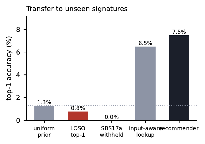
Figure 1. Transfer to unseen signatures. Leave-signatures-out top-1 accuracy is 0.775%, rounded to 0.8% here, below the 1.28% a uniform guess over 78 classes would give, and 0.0% when SBS17a itself is withheld. The probe names the signatures it trained on and fails on the ones it did not.
This is the equivalence from the previous section made concrete. The 0.94 measures the decodable and stops there. The cleaner statement is that centered RSA equals linear CKA, and both equal average linear decoding accuracy over randomized white-noise tasks, so geometry is decodability. That is what the 0.94 measures, and it is why the 0.94 falls short, on its own, of a claim about understanding.
The held-out collapse was one warning among several. I also tested whether simpler properties could reproduce the movement that looked functionally meaningful. A composition-matched control recovered 72% of the steering effect I had measured at one hidden layer, and that ratio is specific to that readout. Log sequence length, fitted across the 78 signatures in one Pfam clan, accounts for R-squared 0.941 of the variation in displacement magnitude, because signatures differ in how often they introduce a premature stop, which changes translated length, which moves a mean-pooled embedding. A strong baseline changes the question. After the composition and length controls, the useful question shifts. It becomes “what residual movement remains after removing simple sequence properties, does it recur across families, and which residues causally carry it?”
The centroid comparison carries its own version of the seed-divergence warning. PRISM measures movement against Pfam centroids, which are category-level summaries. In the same 2020 study, identical CNNs trained from different seeds kept category centroids consistent at about 88% agreement, while the seeds scrambled exemplar-level arrangements inside categories and deep layers showed only 44% consistency across seeds. Training objectives enforce category separation, and they leave internal organization unconstrained. A centroid-level result can therefore look stable while the fine-grained arrangement underneath stays arbitrary, which is one more reason the SBS17a result points at residue-level follow-up work and leaves the question open.
The same pattern appears when a representation becomes a target in place of a measurement. In a separate stress test, learned fitness proxies looked respectable across the full dataset, with Spearman correlation around 0.53. Among the top-ranked variants, where a design system would actually concentrate its effort, utility fell to about 0.15. An unconstrained optimizer pushed the proxy five standard deviations past the natural-protein floor while producing sequences that read as implausible proteins. Average predictive performance and decision quality are different objects. A model can preserve a broad ranking over ordinary examples while giving its largest rewards to pathological ones, and selection pressure turns small blind spots into the entire output distribution.
So I now want three kinds of evidence before I make a strong claim about what a model has learned. Transfer, hold out whole mechanisms, families, environments, or tasks, which blocks a probe from winning by memorizing local fingerprints. Causal intervention, ablate or steer the proposed feature and test whether behavior changes in the predicted direction, which separates readable information from information the model actually uses. Optimization pressure, let selection search against the metric, then inspect top candidates and out-of-distribution behavior, which reveals reward hacking that average scores conceal. These tests are related but distinct, and together they make the claim much harder to fake. A probe should open the next experiment.
Inside a protein language model, where function becomes accessible
The second attempt goes further inside the model. If a probe reading the output embedding is reading the wrong place, then the question is where the right place is. At what depth does intervening along a fitted functional direction move the model’s own output representation, and once the information is there, does it localise into individual sparse features or spread across many?
The functional target is deep mutational scanning fitness across ten ProteinGym assays, 72 to 212 residues. The direction is the difference between mean activations of high- and low-fitness variants, fitted on training proteins only, centred within each protein. Absent that centring, the between-protein offset dominates and the fitted direction becomes a protein detector. I inject the direction with a forward hook at a chosen layer, so the perturbation has to propagate through every remaining layer to reach the readout. Everything then depends on the control. I use three nulls at matched norm, a random Gaussian direction, a direction orthogonal to the fitted one, and the unweighted mean activation. The third is the stiff one, because adding any large in-distribution shift moves embeddings somewhere, and only a control that also moves them tests the hypothesis. That third null is the one I learned to trust, and it is the one that later flipped half my results.
The specific effect is confined to a band near three-quarter depth. Two independently constructed contrasts, built from different definitions of high and low fitness, agree that an interior maximum exists there.
Update, 18 October 2026: I re-ran this wider, and the location did not hold
On roughly double the held-out panel — 22 proteins, 11 test, all 15 layers on an A100 — the number reproduces almost exactly. Restricted to the nine test proteins in the original length range, layer 24 gives +0.0929 against the +0.0933 above. But its interval is [−0.1393, +0.3922], and of the eight layers whose intervals exclude zero, none is in the band.
Two things make it worse. The margin is confounded with how close the injection is to the readout (rank correlation −0.873): a perturbation injected one layer from the output barely has to survive any computation. And under an intervention with no dose parameter, where the displacement comes from real paired variants and every null is held to the same edit magnitude, every band layer has a negative margin, with only depths 0.48 and 0.61 clearing zero.
So the honest version is narrower than the sentence above: a fitted direction beats a generic shift somewhere in the interior, the effect is small, and it resolves nearer half depth. I have left the original claim in place rather than editing it away. This post is about claims that invert once the control is named, and it would be strange to exempt its own.
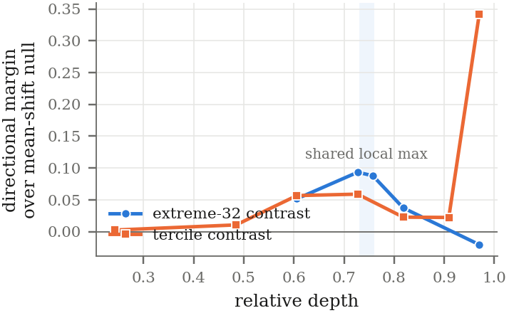
Figure 2. Both constructions find the interior maximum. They disagree in sign about the output region, so I report a band, with no claim about a global optimum.
At the output layer the effect collapses ninety-five-fold in a single layer, from +0.0716 at layer 32 to +0.0008 at layer 33. The cause is architectural. The output passes through emb_layer_norm_after, which removes most of a constant added direction, and the same collapse appears independently in a different target, so it is a property of the architecture. The absolute numbers stay small. The best recovery anywhere is ten percent of the full high-minus-low difference, so any direction I can extract this way leaves ninety percent unreproduced. I stop short of calling this an emergence zone. Five layers of the sweep carry the directional margin and only one carries a protein-level interval, which locates a band. Whether the onset is sharp requires a dense depth sweep with per-protein intervals at every layer, which I have not run.
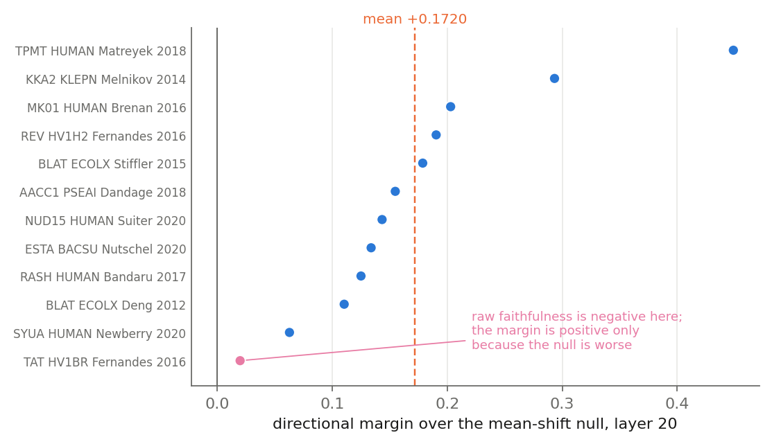
Figure 3. The one cell where I have the full per-protein decomposition. All 12 proteins are positive and the mean is +0.1720, interval +0.1182 to +0.2359. Two things that pooling hides. The margins span a factor of 23, so this is not a uniform property each protein samples with noise. And on TAT_HV1BR the fitted direction moves the representation the wrong way, with the margin positive only because the null moves it further wrong.
The sharpest result is that the null you choose selects your layer, and it is the reason I now distrust my own earlier sweeps. Score the fitted direction the way this literature usually does, against a matched-norm random null, on a distance-to-centroid readout, selecting the layer by significance, and the answer is depth 0.97 at z = 16.24, the largest value anywhere in any sweep I ran. That looks like a discovery. Score the same direction at the same layer against the generic mean-shift null on a directional readout, and its margin is -0.0041. It is worse than an arbitrary shift of the same size. The significant version here is the one I would have reported a year ago.
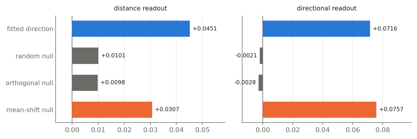
Figure 4. The same cell, four directions, two readouts. On the left the fitted direction towers over the conventional nulls, which is where z = 16.24 comes from, but the mean shift already accounts for two-thirds of the movement. On the right the ordering inverts outright. The null reaches +0.0757 against the fitted direction’s +0.0716.
The mechanism is visible once the stiffer control is in the picture. The conventional nulls miss the generic component of the movement, so a significance score computed against them is largest where that generic component is largest. Each of the three ingredients is ordinary on its own. The combination picks the one layer at which the hypothesis loses to its own control. Three more failures came out of the same sweep, and I report them because each one was mine. First, distance and direction disagree about the same null, at layer 20 the mean-shift null cuts distance by +0.0204, which reads as recovering 48 percent of the effect, while its directional faithfulness is -0.017, slightly anti-aligned. Second, a recovery fraction changes meaning across depths, its numerator grows as the injection point approaches the output while the denominator is fixed, so the same property read 0.11 at depth 0.48 and 1.34 at depth 0.97, and a recovery fraction above one has stopped measuring recovery. Third, a dose-response inside the linear regime proves only linearity, at strengths of 0.5, 1 and 2 the response doubled with every doubling, which established only that the readout is linear in the injected vector.
This is the seed-divergence lesson one level up. In the same 2020 study, identical CNNs trained on CIFAR-10 with the same schedule and sample order diverged under different random seeds, deep layers showed only 44% consistency while category centroids stayed consistent at about 88% agreement, and training objectives leave internal organization unconstrained. Agreement at the coarse level says little about the fine-grained arrangement, and a metric that only sees the coarse level will call two different systems aligned.
If reusable parts carry function, a sparse dictionary should isolate them. I trained a 16,384-feature top-k autoencoder at layer 30, three seeds, 12.8x overcomplete with k = 48 active per residue, and reported held-out quality first, fraction of variance unexplained 0.149, reconstruction cosine 0.914, measured sparsity 48, dead features 2.6 to 3.4 percent. The pre-registered criterion asked for decoder cosine above 0.5 and steering comparable to the supervised direction. In all three seeds the most perturbation-responsive atom is the most decoder-aligned atom, at cosine 0.734 to 0.763. The alignment leg passes and the causal leg falls short. Steering that atom gives -0.0035, +0.0037 and +0.0078 against a supervised reference of +0.0389. The atoms which steer best sit at negative cosine, the opposite sign from where attribution points.
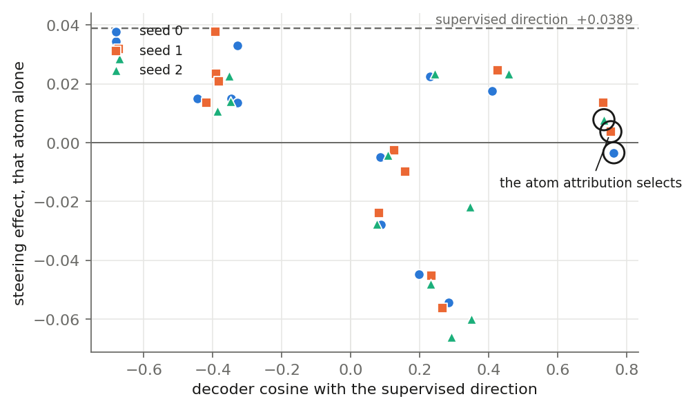
Figure 5. The circled atoms are the ones attribution selects, at cosine around 0.75 and essentially zero steering effect. The atoms that reach the supervised reference sit at negative cosine. Alignment predicts efficacy only weakly, r = +0.445 over 39 candidates.
So the dictionary does contain atoms that realise the direction on their own. The best single atom recovers 86, 95 and 77 percent across seeds. What it lacks is a way to find them from alignment. In every seed the best-steering atom is strongly anti-aligned, at cosine -0.68, -0.39 and -0.67. The sign of the alignment is systematically wrong for the atom that carries the effect, and a mechanism for this escapes me. A related detail bears on any attribution method, seven of the 39 candidates have activation changes indistinguishable from zero, at ranks beyond 15,000 of 16,384, and nonetheless steer at +0.013 to +0.023. A feature the perturbation leaves silent stays invisible to any method based on activation change.
This is the behavioral alignment fallacy in miniature. Identical outward behavior can rest on radically different internal strategies, and standard metrics can report high alignment from superficial correlations. The atom that looks right by alignment and steers at zero is that. The homomorphic encryption result reported in the 2026 eNeuro paper is the same shape, two networks can run identical input-output computation with homomorphically encrypted geometries, giving an alignment score near zero, so representation can be mathematically decoupled from causal computation. Alignment by geometry alone leaves open whether two systems compute the same thing, which is why the steering test carries the weight in this section.
Pooling loses the structure, and the loss is dimensional. For predicting whether an intervention changed the model’s output on held-out proteins, 7,074 training and 1,994 test variants on a protein-disjoint 157/44 split, mean-pooled activations score AUC 0.4931, which is chance, and adding them to the intervention parameters lowers AUC from 0.8338 to 0.6319. The control that makes this readable is a Gaussian random projection at matched dimension, twenty seeds.
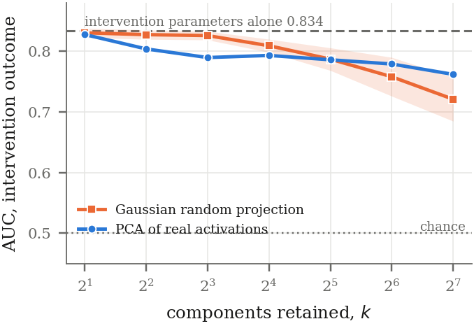
Figure 6. Both curves fall as components are added. The random projection matches the model’s PCA at two components and beats it from four to sixteen, by five standard deviations at eight. Neither reaches the intervention parameters alone.
A random subspace of the same width carries at least as much of what predicts the outcome as the leading principal directions of the model’s activations do. The information is present, the geometry is wrong. Every added direction costs accuracy, which is the signature of a nuisance subspace dominating the variance, and two scalars of boundary margin recover what 1,280 pooled dimensions missed, reaching 0.8846 beside the parameters. Those intervals overlap with the parameters-alone baseline, so I state that as a consistent improvement, short of demonstrated. The geometry caution from the spine applies in full here, with its meeting-note form. Procrustes alignment breaks down across unequal dimensions, 1,000 biological neurons against 10,000 artificial units, and centered RSA equals linear CKA with both equal to average linear decoding accuracy over randomized white-noise tasks, so geometry is decodability. A probe result alone settles what can be decoded, and leaves what a model computes open.
Everything above presupposes that the tests discriminate. For nucleotide models, one of them stays blind. I built a typed-intervention battery the way this literature builds such tests, declare a perturbation, declare the expected direction before scoring, pair within sequence, adjudicate against a reference effect. Reading frame is the natural first property, since a model that represents it should distinguish an in-frame stop codon from the same three bases out of frame. HyenaDNA stays at chance. On 24 coding sequences the frame-anchored stop contrast gives +0.00058, interval -0.00045 to +0.00161, 14 of 24 signed, binomial p = 0.54, which is a coin. An order-0 Markov chain carrying only period-3 structure does pass, at +0.00092, interval +0.00064 to +0.00120, 22 of 24. An order-2 chain passes at six times HyenaDNA’s effect with all 24 sequences signed. An order-0 Markov chain assigns base probabilities that depend only on position modulo three. Its representation stops short of a codon, a stop, or a frame.
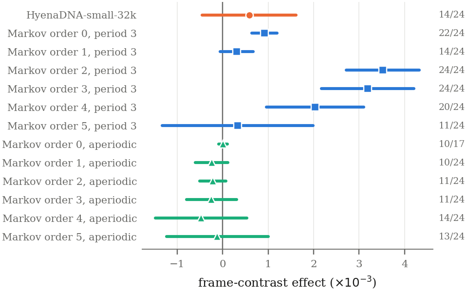
Figure 7. The aperiodic controls locate the problem. Remove the periodicity and keep the model class, and every estimate collapses to zero or inverts. The quantity the test responds to is position-modulo-three periodicity.
Any model with that periodicity scores as representing reading frame, and a model lacking it scores as failing, regardless of whether it represents frame. This stays silent on whether genomic models represent reading frame. It says this test stays blind to the question, and since the test is mine, this is a self-check on my own instrument. The rule I would most want adopted is the one the nucleotide work bought and the protein work missed. Run the test on a model incapable of holding the representation, and report what happens. A null sequence tells you what a given model does on degraded input. A null model tells you whether the test needs the capability it is named for. And one more reason to distrust a bare similarity score here, simplicity bias, means gradient descent prioritizes easily separable, low-frequency linear features over complex nonlinear causal structure, so if a brain and a network both latch onto the same superficial feature, RSA scores high while the model misses the deep causal structure. The control has to remove the easy feature before the similarity means anything.
Reading down the effect column of this work it looks like a set of small positive findings. Reading across to the control column, six of twelve invert. The inversions are mundane, a conventional null, a conventional readout, an unbounded metric, a dose-response inside its linear regime, and each one is individually defensible. The practical version is to put a zero-parameter baseline beside every number. A single unfitted BLOSUM62 feature decodes fitness at 0.165 against ESM-2’s 0.203, and the model’s figure is a maximum over 33 layers chosen on the same held-out proteins it is scored on.
How this sits against the SAE literature
Sparse autoencoders are the standard instrument for asking how a representation is organised, and the bio-foundation-model literature has grown fast enough to have a survey of its own.1 Reading across it, the thing I keep noticing is not the dictionaries. It is what counts as validation.
Table 1 · What each study validates against
| Study | Model | Validated against | Control reported |
|---|---|---|---|
| InterPLM2 | ESM-2 8M–3B | Swiss-Prot annotations, LLM descriptions | annotation overlap |
| Adams et al.1 | ESM-2 650M | InterPro families, coevolution, human preference | annotation overlap |
| Gujral et al.1 | ESM-2 650M | GO enrichment, LLM interpretation | enrichment |
| Parsan et al.1 | ESM-2 3B | UniProt, contact prediction, ESMFold steering | annotation overlap |
| Villegas Garcia & Ansuini3 | ESM-2 8M | Zinc-finger motifs in generated sequences | random latent |
| Guan et al.1 | HyenaDNA-small-32k | JASPAR motifs | annotation overlap |
| This work | ESM-2 650M, HyenaDNA | A measured DMS fitness contrast, reproduced inside the representation | mean-shift null + measured ceiling |
† Validation columns for the studies I did not read end to end are as the survey catalogues them, not as I verified them. The point of the table is the shape of the column, not a score for anyone’s paper.
Almost everything in that last column is an overlap statistic. A feature fires where an annotation says it should, so the feature is given the annotation’s name. That is a real finding about where a feature fires. It is not a finding about whether the model computes with it, and the two come apart more often than I expected: the most decoder-aligned atom in my dictionary, at cosine 0.734 to 0.763, is also the most responsive one, and it carries almost none of the causal effect, while atoms at cosines as low as −0.39 recover 77 to 95 percent of it.†
The survey’s own closing line is that the field still lacks the benchmarks and null models it needs. I read that as the whole problem. Most of what I have built here is null models.
Why a matched-norm random direction is the wrong null
In 1280 dimensions, a random unit vector is close to orthogonal to any fixed target direction. So the expected overlap between a random direction and the real high-minus-low difference is near zero, and almost any fitted direction clears it. Beating a random direction is therefore cheap, and a large margin over one is not evidence of specificity.
The control that actually competes is the generic mean shift: take the unweighted mean activation and inject that. It has the same norm, it is not random, and it carries whatever generic structure the layer has. In my sweep the difference is not cosmetic. Selecting a layer by z-score against the random null picks the single layer where the fitted direction loses to the mean shift, at z = 16.24.
A white-box evaluation for protein models
The third piece is the proposal those two case studies argue for. I want a white-box evaluation for protein models in three parts. Rank fixed sets of already-measured benign variants, recover the assay property with linear probes on internal activations, and hold out whole families to check that the signal transfers. People usually judge a protein model by whether its score correlates with a measured property across a benchmark, and that test can pass for the wrong reason, because the model can rank sequences using a feature that happens to line up with the property on familiar data. A white-box evaluation looks inside the model, and asks whether the property is recoverable from the model’s internal activations and whether that recovery survives a shift to unfamiliar proteins.
The evaluation has three parts that build on each other. First, I assemble fixed sets of protein variants whose properties were already measured in published deep mutational scanning assays, so every label comes from measurement and the design reuses existing sequences only. Second, I train a linear probe, a simple classifier or regressor on a protein model’s internal activations, to recover the assay property, which tests whether the information is present in the representation itself, beyond what the output score shows. Third, I hold out whole protein families, defined by family or clan, during probe training and test on them, so the evaluation measures whether the recovered signal transfers to families new to the probe.
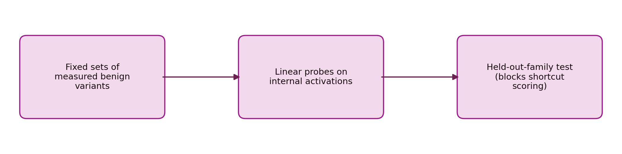
Figure 8. The evaluation runs in three steps, from fixed sets of measured benign variants, to linear probes on the model’s internal activations, to a held-out-family test that blocks shortcut scoring.
The held-out-family split is what makes the evaluation informative, because a probe that reads a shortcut will do well on families it trained on and fall off on new ones. If the probe recovers the property on held-out families, that is evidence the model represents something about the property that generalizes. If the probe falls off, the earlier correlation was standing on family-specific structure, and the score holds only inside its training distribution. This is the same held-out logic that collapsed the 0.94 probe above, promoted from a diagnostic into the design of the evaluation itself.
The proposal is falsifiable. I put the falsifier in first, since my own evaluations have passed for the wrong reason before. If probes recover assay properties just as well on held-out families as on seen ones for a model whose output score is known to shortcut, then the white-box test only reproduces the output correlation. I would report that limit directly, because the point of the evaluation is to detect shortcut scoring, and a version that blurs the two cases falls to its own test.
I state the biosecurity boundary first. I fix the safety boundary before any experiment runs, so the design stays clear of uplift. All of this work uses only benign, already-measured proteins, generates no new functional sequences, runs no wet-lab validation, and releases no reusable steering probe. The output is an evaluation and a report of where a model’s representation carries an assay property and where it falls short, which is a statement about the model. It remains an evaluation, and stops short of a design tool.
What this adds up to
My claim is narrower than a call to replace behavioral evaluation, and I think it is more useful. Behavioral evaluation is necessary and, on its own, structurally insufficient. It will keep breaking under optimization because it reads a projection of the computation. So the evaluations I trust do two things at once. They test the output under the exact pressure the model faces, with trivial baselines and top-tail utility, and they test confound controls and held-out transfer. And they test the computation, asking what is recoverable inside the model and whether it survives a distribution shift.
Reading the computation carries its own risks, and the two case studies are the warning. A probe can hit AUC 0.94 and name only what it trained on. Function can be causally accessible only in a narrow interior band that recovers ten percent of the full effect, the atom that attribution selects can sit at near-zero effect, a pooled embedding can predict intervention outcomes at chance while two scalars do the job, and a Markov chain blind to codons can pass a reading-frame test. Going in, I did not see how much of the work would end up being about the instrument. The z = 16.24 cell is the clearest case, three ordinary methodological choices, each defensible, combining to select the one layer where the hypothesis loses to its own control.
The shared question across all of it, protein design, world models, alignment, is whether an abstraction remains reliable under the pressure created by its use. In protein design that pressure comes from searching sequence space, in an agent from planning over actions, in an evaluation from a system adapting to the score. The domain changes, the evaluation problem is the same. The most important models will move outside the distribution where their scores were calibrated, so the evidence we trust about them has to look past the output, which means building the interpretability tools early, while scores still look healthy, and holding them to the same controls I have had to learn to hold my own to.
References
- Interpreting Bio-Foundation Models with Sparse Autoencoders. Wilber, J. and Shimko, T. NVIDIA Research, 2026. research.nvidia.com — the survey table this post's Table 1 draws its catalogue from.
- InterPLM: Discovering interpretable features in protein language models via sparse autoencoders. Simon, E. and Zou, J. Nature Methods, 2025.
- Interpreting and steering protein language models through sparse autoencoders. Villegas Garcia, E. N. and Ansuini, A. arXiv:2502.09135, 2025.
- The geometry of hidden representations of large transformer models. Valeriani, L., Doimo, D., Cuturello, F., Laio, A., Ansuini, A. and Cazzaniga, A. Advances in Neural Information Processing Systems 36, 2023.
- Estimating the intrinsic dimension of datasets by a minimal neighborhood information. Facco, E., d'Errico, M., Rodriguez, A. and Laio, A. Scientific Reports 7(1):12140, 2017.
- CausalGym: Benchmarking causal interpretability methods on linguistic tasks. Arora, A., Jurafsky, D. and Potts, C. ACL 2024, pages 14638–14663.
- Finding alignments between interpretable causal variables and distributed neural representations. Geiger, A., Wu, Z., Potts, C., Icard, T. and Goodman, N. D. arXiv:2303.02536, 2023.
- Sparse autoencoders trained on the same data learn different features. Paulo, G. and Belrose, N. arXiv:2501.16615, 2025.