How to evaluate AI models for biology

TL;DR. An evaluation of an AI model for biology is a measurement instrument. It outputs a number, and an organization compares that number against a threshold to make a consequential decision, so if the measurement is biased the decision is biased, and if the noise goes unreported a sampling accident can clear or restrict a model. Across protein models, agents, verifiers, and safety benchmarks, the same failure keeps appearing. A score looks healthy on a benchmark and stops meaning anything in the place it is actually used. I think the fix is one idea, applied everywhere. An evaluation is only trustworthy if it still means what it claims once a model or a search optimizes against it, and that is a property you have to test on purpose, with trivial baselines, top-tail utility, confound controls, and held-out transfer, a property those tests establish and a single benchmark number leaves open. This post has two halves that read as one. The first builds the measurement-and-statistics machinery from first principles, separating three estimands that are routinely confused, namely capability, propensity, and uplift, and then assembling the chain from threat model to item to score to interval to decision, covering how to build and grade items, the statistics of a score, item response theory, contamination and saturation, agentic evaluations, randomized uplift trials, decision rules under an explicit burden of proof, an end-to-end pipeline, and reporting under an information hazard. The second runs the battery on live systems in three case studies, a genomic model whose signal a substitution matrix matches, a safety benchmark partly answered from the answer options alone, and a protein-model steering result where the controls took most of the effect. Every statistical number comes from a simulator whose ground truth I know, every evaluation item is a content-free placeholder, and the guide contains no hazardous biological information.

The argument, and why measurement is what matters

When a protein model aces a benchmark, what did we actually learn? For a long time the answer mattered little, because the score was a leaderboard entry. It matters now because the score has become an objective. A lab measures only a fraction of candidates in the wet lab, so it ranks thousands or millions of designs by a computable score and keeps the top ones, and a safety team sets a threshold on a benchmark and treats crossing it as evidence. A proxy is a computable stand-in for a slow measurement, and the moment a search starts choosing the candidates a proxy likes best, the proxy begins to steer the world it once only described. I built this guide around that shift because it is the moment a score stops describing the world and starts steering it.

That shift changes what a good evaluation has to prove. Showing that a score correlates with the truth on ordinary examples now falls short. You have to show that the score keeps its meaning at the exact edge a search selects, and under the exact pressure the model faces.

The same logic drives the safety side, where the stakes are sharpest. Large language models now answer graduate-level biology questions, read and critique laboratory protocols, and operate software tools over long sequences of actions. Science and medicine benefit from most of these capabilities, but a small subset could also lower the barriers that currently stop a person or group from causing deliberate biological harm. Several frontier developers have therefore committed to test each new model for such capabilities before release and to apply stronger safeguards when a model crosses a defined threshold (Anthropic, 2023; OpenAI, 2023; Google DeepMind, 2024). Government institutes run their own pre-deployment tests (US AISI and UK AISI, 2024), and standards bodies have issued guidance on how to measure misuse risk (NIST, 2024). I refer to this body of testing as biosecurity evaluation, and I treat every evaluation for biology, from a protein-fitness proxy to a hazardous-knowledge benchmark, as a measurement instrument. It outputs a number, or a small set of numbers, and an organization compares that output against a threshold to make a consequential decision. If the measurement is biased, the decision is biased. If the measurement is noisy and nobody reports the noise, a sampling accident can clear or restrict a model. Despite these stakes, published evaluations rarely report confidence intervals, rarely state which estimand a test targets, and rarely explain how the team handled refusals, grader errors, or correlated items. Much of this omission is understandable, since evaluation teams work under time pressure and must withhold the hazardous content at the core of many evaluations. As a result, methodological knowledge stays inside a few organizations, and newcomers have to rediscover it.

Prior work covers parts of this ground. The authors of benchmarks such as WMDP (Li et al., 2024), LAB-Bench (Laurent et al., 2024), and the Virology Capabilities Test (Götting et al., 2025) describe how they built and validated individual question sets. RAND (Mouton et al., 2024) and OpenAI (Patwardhan et al., 2024) ran human uplift studies with randomized designs in which participants with and without model access attempt planning tasks. Position papers argue why dangerous-capability evaluations matter and what they should cover (Shevlane et al., 2023; Phuong et al., 2024; Sandbrink, 2023). In general machine-learning evaluation, recent work argues for error bars (Miller, 2024), quantified benchmark variance (Madaan et al., 2024), and applied item response theory to language-model benchmarks (Polo et al., 2024; Rodriguez et al., 2021). Each of these sources covers part of the ground, and the full chain from threat model to item to score to interval to decision, with information hazards as a design constraint on every link, is what this guide assembles.

In this guide I assemble that chain, I introduce each concept with its motivation, derive it in enough detail that a reader can check each step, and implement it in a companion Python library, biosec_eval, in the spirit of tutorial references that pair derivations with working code (Tang, 2025). I test every estimator against data simulated from a known generative model, so the reader can see when a method recovers the truth and when it fails. Then I turn to live systems and run the same battery in full, because the places it breaks are easier to see on a live model than in the abstract.

Three distinctions recur throughout. The first separates what a method measures from what the evidence establishes. The second separates what the evidence establishes from what remains a policy judgment. The third separates results checked here against simulated ground truth from relationships, such as the link between capability scores and uplift, that I treat as assumptions. I assume undergraduate probability and statistics and basic Python, but no background in psychometrics, clinical trials, or biosecurity policy. The rest of this piece first names the ways a score loses its meaning in practice, each one from a measurement I ran, then builds the protocol and the statistics that catch them, then works through the case studies.

A note on scope and safety posture. This guide concerns measurement. It contains no hazardous biological information, and I do not describe how to make any evaluation item more dangerous or more useful to an attacker. Every item in the companion library is a placeholder string such as "Item 0137 (construct C2)", and every response is simulated. Threat models appear as abstract structures with their steps left unnamed. Readers who build their own evaluations should hold their item content under the access controls I describe later.

The core failure is selection on error. Start with the simplest version. Write a score as the true quality plus an error term,

\[s = f^{*} + \varepsilon\]

where the first term is the true quality you care about and the second is the model mistake on that candidate. On an average example the error is just noise and the correlation looks fine. Now let a search look at many candidates and keep the one with the highest score. The kept candidate is the one where the error happened to be most favorable, so the error of the selected item is the maximum of many draws, and

\[\mathbb{E}\big[\max_{i \le n} \varepsilon_{i}\big] \text{ grows with } n.\]

The more you search, the more of the score is error and the less is quality. This is the winner curse, and it is why a proxy that looks healthy in bulk can be useless once you optimize it. It falls out of one line of algebra, and it recurs in places that look unrelated. The same mechanism returns later in two more places, when a safety team reports the best of several elicitation conditions and when a search keeps the top design, so I set out the picture now.

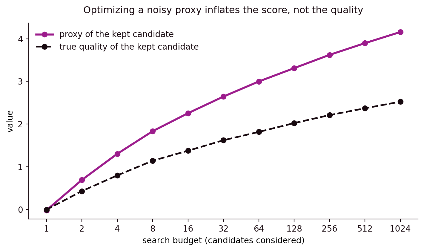
Figure 1. A simulation of the mechanism. Each candidate proxy is its true quality plus independent error, and a search keeps the highest proxy. As the search considers more candidates, the kept candidate proxy climbs steeply while its true quality lags, so the gap between the two is the selected error. This is drawn from Gaussian quality and Gaussian error, and it is schematic.

The practical consequence is that a benchmark’s bulk correlation, a single number across a whole dataset, is measured in the wrong place. Selection happens in the top tail, and that is where you have to look. I tested this directly. I measured whether a scorer benchmark correlation predicts the value of the designs a search actually selects with it. The agreement weakens as selection sharpens, from a squared rank association of 0.50 when keeping the top 10 percent to 0.16 when keeping the top 1 percent, and three of 41 assays give worse-than-random top-1 percent selections despite positive correlations. That last part is the critical one, since a positive bulk correlation is the number a leaderboard would report as healthy.

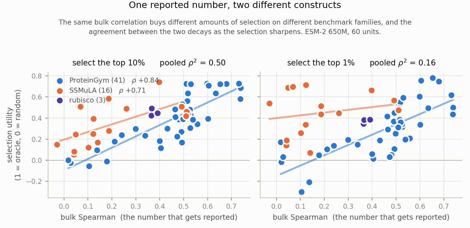
Figure 2. Selection utility against the bulk Spearman that gets reported, on ESM-2 650M. The same reported correlation buys 0.50 of the squared association with selection value at the top 10 percent and only 0.16 at the top 1 percent, and the benchmark family matters more than the score. The recommendation is to report top-k utility and enrichment beyond the bulk correlation.

pause top 100%, variance in selection value explained 0.70

Beyond the top tail, a score has to beat a trivial baseline and survive a confound. Before you credit it with understanding, it has to clear two low bars. It has to beat a trivial baseline, and the part that looks like signal has to survive a control for the obvious confounds. Both bars are easy to state and scores often fail them. On 504 measured PET-hydrolase variants, a zero-shot protein model ranks activity at a Spearman of 0.01 while a plain count of mutations reaches 0.25, so the expensive score adds nothing over counting. I ran this on the 504 measured variants, and the mutation count wins, 0.25 against 0.01.

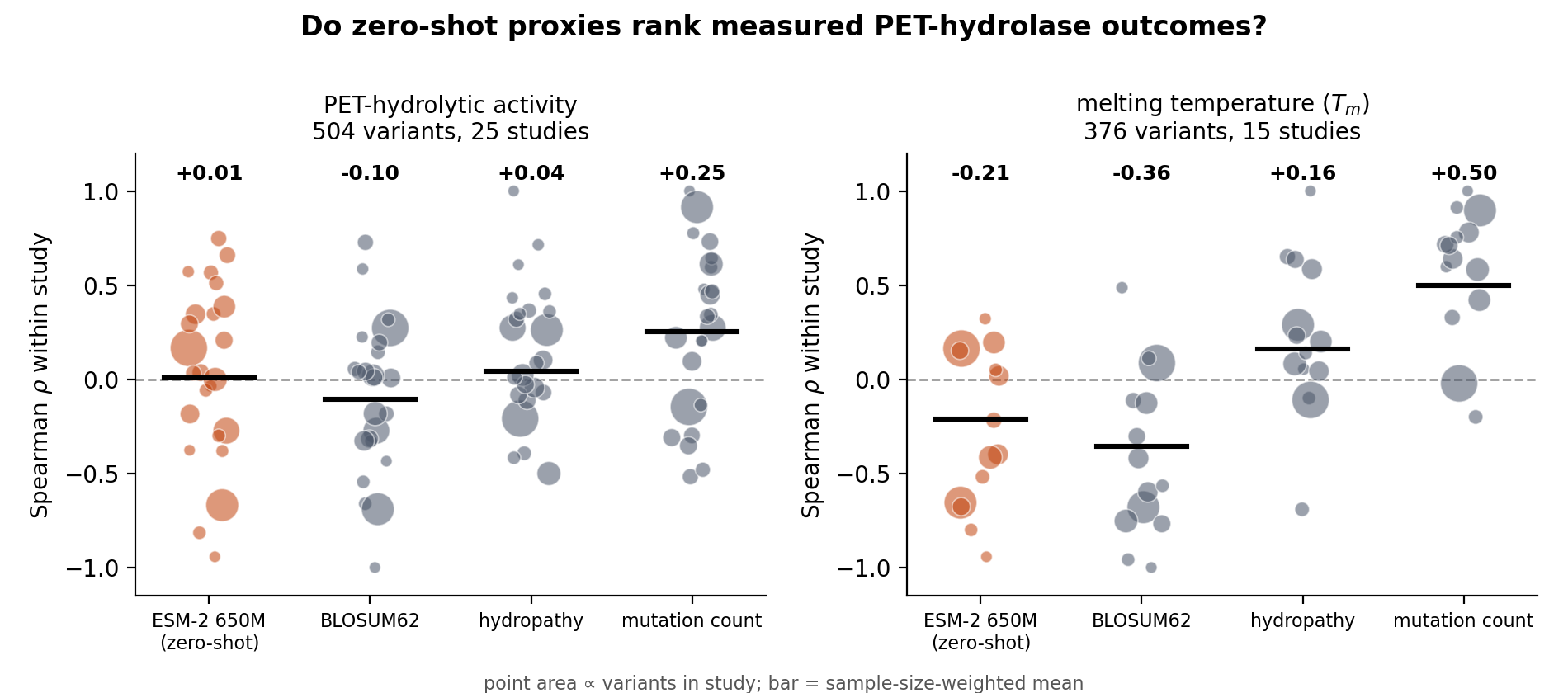
Figure 3. Within-study rank correlation with measured outcomes for four scorers. The ESM-2 650M zero-shot score sits near zero on PET-hydrolytic activity, below a hydropathy feature and well below a mutation count.

The confound control is the other bar. If the plainest property of the input reproduces a movement in a representation, it gives no evidence about the mechanism you are studying. The sharpest version of this I have is the PRISM steering result, where a composition-matched scramble reproduced most of an apparent mutational-signature effect and protein length explained almost all of the displacement magnitude. I work the numbers in the PRISM case study below. The point here is the discipline. Build a control that keeps the confound and destroys the structure you claim, and report the magnitude of what survives, beyond its sign.

In my meeting notes, simplicity bias gives a general reason to expect this kind of failure. Gradient descent prioritizes easily separable low-frequency linear features, such as background color and texture, over complex nonlinear causal structure, as my notes have it. If a brain and a network latch onto the same superficial feature, RSA scores can come out high while the model misses deep causal structure, though I still need to check this before relying on it. That is a false-positive RSA pattern, and it is why a confound control matters even when a similarity score looks strong.

A subtler failure lives at the representation level, where decodability is not understanding. A linear probe is a simple classifier read off a model internal activations, and people take a probe that recovers a concept as evidence that the model represents it. A probe can be right for the wrong reason. The same PRISM work trained a probe to name which mutational process produced an embedding shift, and on processes it saw in training it scored near the top, while on whole processes held out of training it fell below a uniform guess. I read this as the sharpest warning in the whole project, since the same probe looked strong and then fell below chance once I held whole processes out. Those numbers live in the PRISM case study. The general lesson is that decoding and transfer come apart, so decodability is the start of an evaluation, and the held-out test is the end.

In my meeting notes, the behavioral alignment fallacy makes the same point at the level of behavior. Identical outward behavior can rest on radically different internal strategies. Standard neuro-AI metrics can report high alignment from superficial correlations, or so my notes caution, and I have not confirmed it. A probe that decodes well, or a behavior that matches, leaves shared computation unproven. The held-out test is what separates decoding from understanding.

Transfer and scale get overread too. The same caution applies to claims that a model has transferred knowledge or that a capability is scaling. Apparent transfer can be an artifact of how the measurement poses the question. DNA and protein are two encodings of one molecule, so I matched a genomic model and a protein model on the same 25 deep mutational scanning assays. The result, and the control that settled it, is the biologos case study below. The clearest tell was that control. A probe read off genomic embeddings scored about the same after a frameshift destroyed the reading frame, which means it was reading codon identity, well short of protein-level structure.

In my meeting notes, a multimodal grounding study is a useful contrast case for what stronger evidence looks like. Lampinen et al. 2023 tested predictive language processing across 600 human subjects, tracking gaze on paused video clips, in a Visual World Paradigm. Small multimodal models, FLAVA and BLIP, beat massive text-only models, including text-only GPT-4, at predicting human target-word distributions. BLIP layer 9 cross-attention, where text queries attend to visual key and value pairs, accounted for up to 70 percent of human gaze variance. An ablation that shuffled visual attention patches inverted gaze correlation, which points to cross-modal binding. I include those numbers as meeting-notes material, not as my verified results, and they illustrate the bar. A claim of grounding needs a control that breaks the binding, beyond a correlation that survives it.

A last failure appears when the evaluator is the attack surface. So far the model was the thing I measured. In an agent loop the evaluator is itself a component, and a component can be gamed. I red-teamed a verifier, the part that decides which of an agent proposals to keep, in a setting where ground truth exists so I can measure the actual quality of what it keeps. A fully leaked scorer reached an AUROC of 0.991 and added only 0.028 good candidates per batch over random, against 1.082 for a truthful scorer. A scorer this good at discrimination adds almost nothing to the value of what it kept. Worse, a probe that spot-checks a quarter of decisions detects 99.2 percent of attacks and recovers only about 10 percent of the lost value when its fallback is random selection, so catching an attack and undoing it are different things. Getting to 17 percent needs a second source of capability beyond the attacker’s control, a model trained on the campaign own measurements, which is a different fix from the detector.

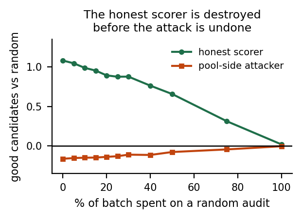
Figure 4. Good candidates per batch over random, against the share of the batch spent on a random check. The truthful run loses value to the check faster than the check recovers from the attacked one, so detection and recovery are different quantities and a report must give them separately.

Those are the failure modes, each one from a measurement I ran. The rest of this guide builds the measurement and statistics that catch them, starting with notation and the decision to work entirely in simulation, and the full battery returns as a checklist once the machinery is in place.

I use one set of symbols throughout. Items are indexed by \(j = 1,\dots,n\), respondents (models or human participants) by \(r = 1,\dots,R\), and repeated samples of the same respondent on the same item by \(s = 1,\dots,K\). When items share a scenario, I call the scenario a cluster and index it by \(c\), with \(m_{c}\) items in cluster \(c\). The graded outcome of sample \(s\) of respondent \(r\) on item \(j\) is \(y_{rjs} \in \{0,1\}\), the per-item mean over its \(K\) samples is \(\bar y_{j}\), the benchmark score is \(\hat\mu\), and the estimand it targets is \(\mu\). The intraclass correlation of outcomes within a cluster is \(\rho\). In item response theory, \(\theta_{r}\) is the latent ability of respondent \(r\), and \(a_{j}, b_{j}, c_{j}\) are the discrimination, difficulty, and guessing floor of item \(j\), with Fisher information \(I_{j}(\theta)\). A grader has sensitivity \(\mathrm{Se}\) and specificity \(\mathrm{Sp}\). In an uplift trial, \(p_{0}\) and \(p_{1}\) are the control and treatment success probabilities and \(d\) is the standardized mean difference. The decision threshold is \(\tau\), the type I error rate is \(\alpha\), and the power is \(1-\beta\), with \(z_{q}\) the \(q\) quantile of the standard normal distribution.

A hat denotes an estimate, so \(\hat\mu\) estimates \(\mu\), and \(\operatorname{SE}(\cdot)\) is a standard error. Confidence intervals are two-sided at the 95 percent level unless stated otherwise. The field overloads the word model, which can mean the AI system under test or a statistical model of responses. To keep these apart, I call the AI system the model under test, or the respondent when the statement applies equally to humans, and I call statistical models by their names, for example the 2PL model.

The companion library depends only on NumPy, SciPy, and Matplotlib, and its modules follow the structure of this guide, items, simulate, grading, stats, irt, agentic, contamination, robustness, uplift, thresholds, harness, and reporting. Two scripts reproduce every number and figure, with all random seeds fixed.

Why simulation. I use no actual evaluation data, for two reasons. The first is safety. Actual biosecurity items and transcripts are information hazards, and publishing them would defeat the purpose of the evaluation. The second is methodological. When data come from a simulator with known parameters, I can check whether an estimator recovers those parameters. I built all of it on simulation for this reason, so I can see when a method recovers the truth and when it fails. For example, I can test a confidence interval that claims 95 percent coverage by drawing thousands of benchmarks and counting how often the interval contains the truth. A single actual benchmark, where the truth is unknown, rules out such a check. The simulators generate realistic structure while holding all content out. Items vary in difficulty and discrimination, items within a scenario share a difficulty offset, multiple-choice items have a guessing floor, refusals can depend on the item, and human participants vary in baseline skill.

What a biosecurity evaluation measures

An evaluation produces a number, and a decision rests on that number. Before asking whether the number is precise, I have to ask what quantity it estimates. This section defines the quantities that biosecurity evaluations target, explains how a threat model fixes those quantities, and introduces the two constraints that shape every later design choice. Validity asks whether a score supports the inference drawn from it, and the information hazard comes from the evaluation’s own content.

Three estimands: capability, propensity, and uplift

An estimand is the quantity an evaluation tries to learn. Biosecurity evaluations target three different estimands, and confusing them frequently leads to misread results. Consider a model under test \(M\) and a task \(T\) drawn from a population \(\mathcal{T}\). Write \(Y(M, T, e) \in \{0,1\}\) for whether \(M\) completes \(T\) successfully under an elicitation configuration \(e\), where \(e\) includes the prompt, the sampling temperature, any tools, any scaffolding, and any fine-tuning applied before the test.

The capability of \(M\) is the success rate under the best elicitation available to a relevant actor,

\[\mu_{\text{cap}}(M) = \max_{e \in \mathcal{E}} \; \mathbb{E}_{T \sim \mathcal{T}}\big[ \Pr(Y(M,T,e) = 1) \big],\]

where \(\mathcal{E}\) is the set of elicitation configurations a relevant actor could plausibly use. Capability answers what the model can do, and the maximum carries weight. A model that fails under a plain prompt but succeeds with a better prompt or with tools has the capability, so a measurement under the plain prompt underestimates it.

The propensity of \(M\) is the success rate under the configuration users actually encounter, usually the deployed system with its safeguards,

\[\mu_{\text{prop}}(M) = \mathbb{E}_{T \sim \mathcal{T}}\big[\Pr(Y(M,T,e_{\text{deploy}}) = 1)\big].\]

Propensity answers what the deployed system will do when asked. A model with high capability and low propensity has the knowledge but refuses to share it. Safeguard evaluations, including tests against adversarial prompting (Wei et al., 2023; Zou et al., 2023), estimate how far a determined user can push the propensity toward the capability.

The uplift of \(M\) for a population of human actors \(\mathcal{H}\) is the causal effect of model access on their success,

\[\Delta(M) = \mathbb{E}_{H \sim \mathcal{H},\, T \sim \mathcal{T}}\big[ \Pr(Z(H, T, M) = 1) - \Pr(Z(H, T, \varnothing) = 1) \big],\]

where \(Z(H,T,M)\) is whether actor \(H\) succeeds with access to \(M\), and \(Z(H,T,\varnothing)\) is the counterfactual with only the resources the actor would otherwise have, such as internet search and textbooks. Uplift answers the question most risk policies care about, namely whether the model makes harmful outcomes more likely than a world without it.

Each of the three quantities is a property of a model together with its measurement conditions. Capability is defined relative to an elicitation set \(\mathcal{E}\) and a task population \(\mathcal{T}\), and a larger \(\mathcal{E}\) can only raise the maximum, so two capability estimates made with different elicitation sets stand on different scales. Propensity is defined relative to one deployment configuration and changes whenever the system prompt, the safeguards, or the user interface change. Uplift is defined relative to an actor population, a task population, a control condition, and an outcome, and changing any of these four changes the estimand. Every report should therefore give each number as “the capability of \(M\) on \(\mathcal{T}\) under \(\mathcal{E}\)” or “the uplift of \(M\) for \(\mathcal{H}\) on \(\mathcal{T}\) against \(\varnothing\),” and state each scope explicitly.

The three estimands are related, yet each stands independent of the others. A model can score well on a knowledge benchmark, a capability measurement, and give no uplift, because the same knowledge is equally easy to find online. A model can give uplift while scoring low on benchmarks, for example by helping a novice organize public information or troubleshoot an error. Sandbrink (2023) draws a related distinction between language models, whose main risk is broadening access to existing knowledge, and specialized biological design tools, whose main risk is raising the ceiling of what an expert can do.

Each estimand needs a different study design. Running the model on a set of items measures capability and propensity, which is cheap and repeatable. Uplift needs a randomized trial with human participants, which is expensive and slow. In practice organizations run capability evaluations often as early-warning signals and run uplift studies rarely to calibrate what capability scores mean (Patwardhan et al., 2024; Mouton et al., 2024).

The proxy assumption. Capability thresholds in published safety policies act as proxies for uplift thresholds. I treat that relationship as an assumption, and I know of no study that establishes a general quantitative relationship between benchmark capability and human uplift. A qualitative argument suggests when the proxy is reasonable. If no elicitation in \(\mathcal{E}\) draws the information or help a step requires out of a model, then a human working through the same channels draws none either, so low capability on a step implies low uplift on that step. The argument depends on three conditions. The task population must cover what the actor would actually ask, the elicitation set must include what the actor could actually do, and uplift must come from content the model produces, beyond encouragement, time savings, or help organizing a search. When any condition fails, low capability stops bounding uplift. High capability leaves uplift open, because the actor may struggle to recognize correct answers, or may find the same information elsewhere at equal cost.

As an example, suppose a developer reports that a model scores 0.62 on a knowledge benchmark and that domain experts score 0.40 on the same items. This is a capability statement. It leaves open whether the model would help a non-expert because non-experts may struggle to recognize which answers are correct, and it leaves open whether the deployed model would share the information because safeguards may block the relevant requests. Each further claim needs its own evidence.

Threat models as measurement specifications

A threat model describes a pathway by which a model could contribute to harm. Risk policies usually state threat models in terms of an actor and a degree of contribution (Anthropic, 2023; OpenAI, 2023; Google DeepMind, 2024). For measurement, a threat model has three jobs. It fixes the actor population \(\mathcal{H}\), which determines whom an uplift trial should recruit; it fixes the task population \(\mathcal{T}\), which determines what the items should test; and it fixes the elicitation set \(\mathcal{E}\), which determines how hard evaluators must try to draw out the capability.

Harmful biological outcomes require a sequence of steps, and an actor fails if any required step fails. Public analyses describe this structure at a high level and leave the operational detail of the steps unstated (National Academies, 2018; Mouton et al., 2024; Carter et al., 2023). I represent the structure abstractly. Let a pathway consist of steps \(1, \dots, S\), and let \(q_{s}\) be the probability the actor completes step \(s\) given earlier steps succeeded. If all steps must succeed, the end-to-end success probability is

\[P_{\text{end}} = \prod_{s=1}^{S} q_{s}.\]

Writing \(q_{s}^{(1)}\) for the step probability with access and \(q_{s}^{(0)}\) without, the end-to-end uplift ratio is

\[\frac{P_{\text{end}}^{(1)}}{P_{\text{end}}^{(0)}} = \prod_{s=1}^{S} \frac{q_{s}^{(1)}}{q_{s}^{(0)}}.\]

This has two consequences. First, a model that helps with one step has limited effect if a different step stays very hard, the bottleneck or weakest-link property. If the threat model correctly identifies which step most limits success, concentrating evaluation there gives the most information per item; if it misidentifies the bottleneck, that concentration leaves the actual bottleneck untested. Second, the effect of a model multiplies across steps, so modest help on several steps can compound into a large end-to-end change, and evaluations that test each step in isolation can miss this compounding. I leave the bottleneck for each actor class unidentified; that mapping belongs to the threat model, held at its own tier.

A biosecurity evaluation should have a test blueprint derived from its threat model, a table whose rows are the steps or capabilities the threat model identifies as relevant and whose entries record how many items, of which formats, at which hazard tiers, target each row. The blueprint makes an evaluation’s coverage claims auditable, so a reviewer can tell whether a high or low score reflects the model or an unbalanced item set.

Constructs and validity

Validity belongs to an inference, and a test holds validity only in relation to one. Psychometricians call the unobserved attribute a test tries to measure a construct, for example “ability to troubleshoot a failed laboratory procedure of a given class.” We observe only item responses, and we infer the construct from them. Cronbach and Meehl (1955) introduced construct validity, and Messick (1995) later argued that validity is a single, unified judgment about whether the evidence supports the interpretations and uses of a score. I adapt four kinds of evidence.

Content evidence asks whether the items cover the construct as defined by the threat model and avoid a different construct; the test blueprint is the main tool. Response-process evidence asks whether respondents answer by using the construct or by some other route, such as eliminating implausible distractors or recalling an item verbatim from training data. Criterion evidence asks whether the score predicts an external outcome that matters, and for biosecurity the most relevant criterion is uplift, so the strongest validity evidence for a capability benchmark is a demonstrated relationship between benchmark scores and uplift-trial results. Because uplift trials are expensive, such evidence is scarce, and when it is missing the link from score to risk rests on expert judgment, which reports should say. Consequential evidence asks what happens when the score is used. A threshold that is too strict delays useful models, one that is too lenient releases risky ones, and a benchmark that becomes a training target loses its meaning. The response-process and criterion questions are where the case studies later in this guide do their work, since a probe that decodes a concept and a score that correlates in bulk are both response-process claims that a held-out control can overturn.

Ecological validity describes how closely the test conditions match the conditions of actual use, and biosecurity evaluations face a structural limit on it. The conditions of concern involve physical laboratory work, which evaluations of software systems hold outside their scope by necessity and by design. Every evaluation therefore measures a proxy, and the gap between the proxy and the actual task is a permanent source of uncertainty that reports should state explicitly.

A taxonomy of evaluation types

Biosecurity evaluations fall into a small number of design families, and each family gives a partial picture, so published assessments combine several (Anthropic, 2025; US AISI and UK AISI, 2024; Phuong et al., 2024). Multiple-choice knowledge benchmarks (Li et al., 2024; Götting et al., 2025) target capability at low cost but are vulnerable to the fact that recognizing an answer among four options is easier than producing it and much easier than the corresponding laboratory work, along with guessing, distractor artifacts, and contamination. Open-ended written tasks such as protocols and troubleshooting (Laurent et al., 2024) come closer to the skill of interest but need graders whose reliability becomes part of the measurement. Agentic tasks with tools (Kinniment et al., 2023; Kapoor et al., 2024) measure persistence and recovery from errors but are expensive to build and vary across runs. Safeguard and red-team tests (Ganguli et al., 2022; Perez et al., 2022) target propensity. Human uplift trials (Mouton et al., 2024; Patwardhan et al., 2024) measure the causal estimand directly but cost the most and are hardest to power. Biological design tool evaluations (Sandbrink, 2023) raise in-silico-proxy and very-high-hazard-output concerns of their own.

Information hazards and the measurement paradox

Bostrom (2011) defined an information hazard as a risk that arises from the spread of true information, and Lewis et al. (2019) applied the idea to biotechnology. Biosecurity evaluations face a sharp version I call the measurement paradox. Content validity requires items that probe the steps of concern, and items that probe those steps, together with their answer keys and the transcripts they elicit, are themselves potentially useful to an attacker. The more valid the evaluation, the more hazardous its contents.

The paradox resists a full solution, and I manage it in four parts. First, tier every artifact. Each item, answer key, rubric, and transcript receives a hazard tier that determines who may access it and travels with the artifact through every stage. Second, separate content from measurement. The statistical machinery needs only graded outcomes, item identifiers, and metadata, so content can stay in a secure environment while only outcomes leave it. Third, prefer proxies at the lowest sufficient tier, since many constructs can be measured with items less hazardous than the actual task but requiring the same skill. Fourth, report aggregates with suppression, coarsening published results and suppressing any slice so small it would reveal individual items. These practices also protect validity, because a benchmark whose items leak onto the internet will eventually appear in training data, and scores on it will then reflect memorization.

The companion library encodes tiers as an ordered enumeration, from PUBLIC (may be released verbatim), through CONTROLLED (shared with vetted evaluators under agreement) and RESTRICTED (held by the item owner; only aggregate scores leave), to WITHHELD (not written down outside a secure environment). Because the tiers are comparable integers, code can compute the maximum tier of a collection, which sets the handling requirements for any derived artifact such as a full transcript log. Each item can return a redacted view for ordinary logs, replacing its content with a stable fingerprint, a truncated SHA-256 hash that lets two parties confirm they evaluated the same item while keeping its text hidden. For restricted items the deployment should compute this fingerprint with a secret key, since a truncated hash of a short text can be broken by guessing candidate texts.

Building and grading items

An item is the smallest unit of an evaluation, a prompt, a way to grade the response, and metadata that tells the analysis how the item relates to others. Errors at the item level propagate into every later calculation, and statistics leave many of them in place afterward. In the companion library each item records its construct (which links it to a blueprint row), format, stem, tier, choices and answer key, rubric, cluster (which items share a scenario or source document), author, creation date (for temporal contamination tests), and the rate at which independent experts agreed with the key (which bounds the attainable score). A blueprint turns a threat model into item counts, and the first quality-control step compares realized coverage against it, by items and by clusters, since a construct with many items but only two clusters behaves like a construct with few items.

Writing items without writing hazards

For a given construct, item writers can consider an abstraction ladder ordered by how close items are to the hazardous task. The top rung is the task itself, which nobody writes down, and the handling environment caps the ladder. The guiding principle is to choose the lowest rung at which the item still measures the construct. Whether a lower rung is valid is an empirical question, and you test it by checking whether scores on low-rung items predict scores on a small, tightly controlled set of higher-rung items.

Domain experts should write the items, and different experts, outside the set who wrote them, should validate them, recording per item the rate at which validators agree with the key. Rein et al. (2023) introduced a useful check for knowledge items, in which skilled non-experts with web access attempt each item and the team flags items they answer easily as searchable; because this exposes item content, it should run only at the CONTROLLED tier or below, with a retrieval-only proxy inside the secure environment for higher tiers. Weak distractors make items easier than intended, so after a pilot one can check how often respondents choose each distractor, since a distractor nobody chooses lowers the effective number of options and raises the guessing floor. Published benchmarks contain a non-trivial fraction of wrong answer keys (Northcutt et al., 2021; Gema et al., 2024), and for strong models wrong keys become the main remaining source of errors, so at least two independent experts should review each item, and the team should remove or rewrite disputed keys.

Multiple-choice items

A multiple-choice score depends on how the evaluation parses answers, on the order of the options, and on the guessing floor. A language model returns free text, so the evaluation must extract a choice from it, and the evaluation must keep parsing failures separate from wrong answers and refusals. The library’s parser prefers an explicit answer line and otherwise takes the last standalone letter, because models usually restate options while reasoning before committing at the end. Whatever rule you use, the report should give the parse-failure rate per model, since a high rate means the evaluation partly measures formatting behavior.

Language models show position preferences in multiple-choice questions, favoring some letters regardless of content (Zheng et al., 2024). The remedy is to shuffle option order independently for each sample and map the parsed letter back to the underlying option, recording the permutation so the analysis can estimate position effects afterward. A respondent who guesses uniformly among \(k\) options scores \(1/k\) on average, so you can rescale a raw score so chance maps to zero and perfect to one,

\[\hat\mu_{\text{corr}} = \frac{\hat\mu - 1/k}{1 - 1/k}.\]

This assumes a respondent either knows the answer or guesses uniformly; partial knowledge violates it, which the 3PL model handles more flexibly with a per-item floor. Reports should say whether scores are corrected. The subtler danger is that the options themselves carry information beyond the construct, since a distractor that is systematically shorter or worded differently from the key lets a model, or a trivial rule, score above chance from the options alone. The next case study measures that leak on a published safety benchmark.

Open-ended items and rubric grading

Open-ended items ask the respondent to produce an answer, such as a written protocol or a diagnosis of a failure, and need a grader. A rubric breaks grading into a list of criteria marked met or not met, some of them critical, so that a response missing a critical criterion fails regardless of the rest. The rubric score is a weighted fraction in \([0,1]\), and whether to report it continuously or threshold it into pass and fail depends on the construct.

Because human experts grade slowly and at high cost, evaluations increasingly use a language model as a grader (Zheng et al., 2023). Judges introduce their own errors and biases, including position bias and a preference for longer answers. Two design choices reduce the problem. The judge should grade one rubric criterion at a time, since a narrow binary question is easier to answer reliably than a global score, and the team should measure the judge’s accuracy on a gold set of human-labeled responses and use it to correct the final rate. The library’s judge template passes the response by reference, so the secure environment resolves the reference and ordinary prompt logs stay free of restricted transcripts.

Refusals and the estimand

How you score a refusal decides which estimand the score targets, and every choice carries a consequence. Scoring refusals as incorrect makes the score estimate propensity, since a refusal is an actual outcome a user would face. Scoring them as missing and computing the score over answered samples estimates capability conditional on answering, which is an estimate of capability only if refusals are unrelated to whether the model would have answered correctly. Dropping every item with any refusal changes the item population and is rarely appropriate.

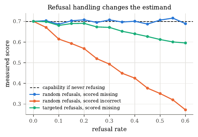
Figure 5. Refusal handling changes what a score measures. A simulated model with true capability 0.70 (dashed line) refuses a growing fraction of samples. When refusals are random, scoring them as missing recovers the true capability, while scoring them as incorrect measures propensity and falls with the refusal rate. When refusals target the items the model finds easiest, scoring them as missing is biased downward because the refused items form a biased subset.

In practice you resolve this by measuring capability on a configuration that answers every item, so the refusal policy drops out of the capability estimand. Developers usually have access to helpful-only model versions that forgo safety training for this purpose, and capability evaluations in published system cards use such versions (Anthropic, 2025). The team then measures propensity separately on the deployed configuration, with refusals scored as non-success. External evaluators with access only to the deployed model can measure propensity but can only bound capability. Refusal detection itself makes errors, missing partial compliance and flagging benign hedging, so a team should audit any detector against human labels and report its error rates.

Grader agreement

Agreement between graders limits how well any score can measure the construct, and raw percent agreement overstates reliability because some agreement happens by chance. If 90 percent of responses fail, two graders who each mark responses as failing at random 90 percent of the time agree on \(0.9^2 + 0.1^2 = 0.82\) of responses from chance alone. Cohen (1960) corrected for this. Let \(p_{o}\) be observed agreement and let the agreement expected under independent labeling with the observed marginal rates be

\[p_{e} = \sum_{k} \pi_{A,k}\,\pi_{B,k}.\]

Cohen’s kappa is the fraction of possible improvement over chance that is achieved,

\[\kappa = \frac{p_{o} - p_{e}}{1 - p_{e}}.\]

Kappa equals 1 for perfect agreement, 0 for chance agreement, and turns negative for systematic disagreement. The conventional verbal labels for kappa values (Landis and Koch, 1977) are arbitrary, and a team should keep them out of pass criteria. For several graders who each label a different subset, Krippendorff (2004) defined an agreement coefficient \(\alpha = 1 - D_{o}/D_{e}\) that handles any number of graders and missing labels. When graders give continuous scores, you measure agreement with an intraclass correlation coefficient, usually ICC(2,1) (Shrout and Fleiss, 1979), which treats both responses and graders as random and penalizes graders who differ systematically in leniency,

\[\mathrm{ICC}(2,1) = \frac{MS_{R} - MS_{E}}{MS_{R} + (k-1)MS_{E} + \tfrac{k}{n}(MS_{C} - MS_{E})}.\]

A design detail prevents a common confound. If grader \(A\) scores all responses from model \(X\) and grader \(B\) all responses from model \(Y\), any difference in leniency appears as a difference between the models. Each grader should score responses from every model, in random order, blind to which model produced which response. This is the evaluation analogue of blinding in a clinical trial.

Correcting pass rates for grader error

An imperfect grader biases the observed pass rate toward its own error rates, and if the grader’s sensitivity and specificity are known you can remove the bias. Let \(\pi\) be the true pass rate, with judge sensitivity \(\mathrm{Se} = \Pr(\text{judge pass} \mid \text{true pass})\) and specificity \(\mathrm{Sp} = \Pr(\text{judge fail} \mid \text{true fail})\). The probability the judge marks a random response as passing is

\[\pi_{\text{obs}} = \pi\,\mathrm{Se} + (1-\pi)(1 - \mathrm{Sp}),\]

which is linear in \(\pi\), and solving gives the Rogan-Gladen estimator (Rogan and Gladen, 1978),

\[\pi = \frac{\pi_{\text{obs}} + \mathrm{Sp} - 1}{\mathrm{Se} + \mathrm{Sp} - 1}.\]

The denominator \(\mathrm{Se} + \mathrm{Sp} - 1\) is Youden’s \(J\) statistic, which is zero for a judge no better than chance, in which case the observed rate carries no information. A judge with imperfect specificity inflates low pass rates, which is where biosecurity evaluations often operate, so specificity carries the most weight. In the verification run, a true pass rate of 0.12 graded by a judge with sensitivity 0.85 and specificity 0.95 shows as 0.146, and the correction recovers 0.12. I run this correction whenever a judge model grades, because the naive rate of 0.146 sits far from the true 0.12 at low pass rates.

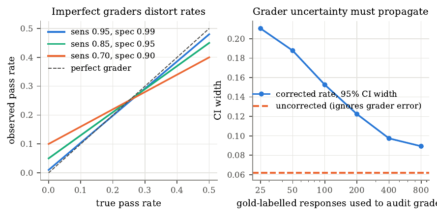
Figure 6. Grader error and its correction. Left, observed pass rate as a function of the true rate for three judges; imperfect specificity inflates low rates. Right, width of the 95 percent interval for the corrected rate as the gold set used to audit the judge grows, for an observed rate of 73/500. The dashed line shows the width of a naive interval that ignores grader error.

In practice you estimate \(\mathrm{Se}\) and \(\mathrm{Sp}\) by comparing the judge with expert labels on a finite gold set, so the corrected rate inherits uncertainty from the observed rate and the two estimated grader rates. A parametric bootstrap propagates all three by drawing each from a Beta posterior and applying the correction to each draw. With a gold set of 25 responses the corrected interval is more than three times as wide as the naive interval, and even with 800 gold responses it stays wider, because the naive interval leaves out an actual source of uncertainty. Evaluations that use judge models should report the gold-set size, the estimated sensitivity and specificity, and an interval that includes grader uncertainty. The correction also assumes the judge’s error rates are the same for every model, which can fail if a judge is more lenient toward responses in its own style, so the gold set should include responses from each model.

Case study, a safety benchmark answered without the question

The item-level artifacts above are not hypothetical. Safety benchmarks inherit every one of these failures, and the stakes are higher because thresholds are keyed to them. WMDP-Bio is a multiple-choice benchmark meant to measure hazardous biology knowledge, and each of its 1,273 items has four answer options. I wanted to know how much of the score a model could earn from the answer options alone, so I ran baselines that see only the answer options. The longest-answer rule takes the option with the most characters and breaks ties by position. The question-blind classifier is a logistic regression on the option text alone, scored with grouped cross-validation so that no question-similarity cluster lands in both the training and the test split.

Random guessing on four options scores 25 percent. Always choosing the longest answer scores 46.5 percent, which is 21.5 points above chance from a rule that uses no biology. A rule this blunt lands 21.5 points above chance on a benchmark meant to gate safety decisions. A cluster bootstrap over 1,195 question-similarity groups puts the guessing-corrected solvable fraction at 0.287 in an interval of 0.249 to 0.324, and the interval for the longest-answer rule itself excludes chance. The mirror case confirms the mechanism. Always choosing the shortest option scores 0.153, below chance, because correct answers here are systematically longer.

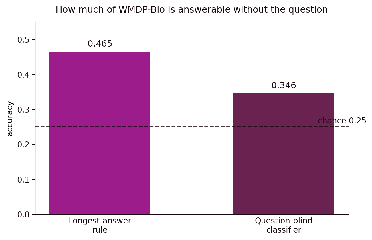
Figure 7. Accuracy of two question-blind rules against the 0.25 chance line. The longest-answer rule scores 0.465 and the question-blind classifier 0.346, and both intervals exclude chance on a cluster bootstrap.

The longest-answer rule tests one artifact. The question-blind classifier tests whether the answer options carry other cues, so I trained it on the options alone. It reached 34.6 percent, which is 9.6 points above chance from the options alone, and its interval also excludes chance. I also checked whether it is only reading answer length. I ran this check because I thought the whole leak was answer length, and on a subset built so that every length rule scores at chance, the option-only logistic regression still reaches 0.325, so part of the signal sits in how the correct answer is written, beyond its length.

These baselines stop short of showing that WMDP-Bio measures nothing. They show that a score on it mixes biological knowledge with artifacts in how the answer options were written, so a model’s score is an upper bound on what it knows until you subtract the artifact share. Against a reference of all 57 MMLU subjects run through the same battery, WMDP-Bio sits at the 96.5th percentile on option-only solvability, with two subjects above it. WMDP-Bio shares this flaw with others. It carries one of the largest of these artifacts and, at 1,273 items, the best-measured one. The open question is whether models actually use these cues when they answer. That needs model weights and a separate measurement, which I have not run, so nothing here shows that any model scores on WMDP-Bio by picking long answers. What the baselines establish is only that the benchmark leaves that door open, and that any threshold keyed to a WMDP-Bio score inherits the artifact until it is controlled. It is a response-process failure of the kind the validity section warned about. A respondent answers the item through a route outside the construct’s intent.

The statistics of a benchmark score

A benchmark score is an estimate built from a finite set of items, a finite number of samples per item, and a grader with some error rate. A different but equally valid set of items would have produced a different score. Miller (2024) treats many of these ideas compactly for general language-model evaluation, and I extend that treatment with derivations and with the clustered and repeated-sampling cases that biosecurity benchmarks often have.

What the score estimates

The items in a benchmark are a sample from a larger population of items that could have been written to test the same construct. Let item \(j\) have true success probability \(p_{j}\), the long-run fraction of correct samples. The benchmark score with \(K\) samples per item is

\[\hat\mu = \frac{1}{n}\sum_{j=1}^{n} \bar y_{j}, \qquad \bar y_{j} = \frac{1}{K}\sum_{s=1}^{K} y_{js}.\]

The fixed-item estimand is the mean of \(p_{j}\) over the \(n\) items actually in the benchmark, with uncertainty only from sampling the model. The item-population estimand is \(\mu = \mathbb{E}_{j}[p_{j}]\) over the population the benchmark was drawn from, with uncertainty from sampling both the model and the items. For biosecurity I usually want the item-population estimand, because the decision depends on the construct and the particular items only stand in for it. Once you adopt that estimand, the standard error must include between-item variance, and you must compare two models on the same items so that item-sampling variance cancels. There is a subtler version of the same warning, which the case study at the start of this guide made concrete. A benchmark’s bulk correlation is itself a statistic measured over the whole item population, and it can miss the top tail where a search actually selects, as Figure 2 and the decay animation show.

Intervals for a proportion

Consider \(n\) independent items, one sample each, with \(k\) correct, so \(k \sim \text{Binomial}(n, \mu)\) and \(\hat\mu = k/n\). The textbook Wald interval

\[\hat\mu \pm z_{1-\alpha/2}\sqrt{\frac{\hat\mu(1-\hat\mu)}{n}}\]

performs poorly near 0 or 1 and for small \(n\); at \(\hat\mu = 0\) it has zero width and claims certainty from a handful of failures (Brown et al., 2001). Biosecurity evaluations often produce scores near 0 or near 1, where Wald fails. Wilson (1927) inverts the score test instead, collecting every \(\mu_{0}\) the test retains, which gives endpoints

\[\frac{1}{1 + z^2/n}\left[\hat\mu + \frac{z^2}{2n} \pm z\sqrt{\frac{\hat\mu(1-\hat\mu)}{n} + \frac{z^2}{4n^2}}\right].\]

The Wilson interval pulls its center toward \(1/2\), keeps positive width at \(\hat\mu = 0\), and holds close to nominal coverage. Clopper and Pearson (1934) instead guarantee at least nominal coverage by inverting exact binomial tests, with limits written as Beta quantiles \([\,B_{\alpha/2}(k, n-k+1),\; B_{1-\alpha/2}(k+1, n-k)\,]\); the guarantee costs some conservatism, so I use it when a decision rule needs a guaranteed bound.

As an example, a model that succeeds on 0 of 30 agentic tasks has a Wald interval of \([0,0]\), a Wilson interval of \([0, 0.114]\), and a one-sided 95 percent Clopper-Pearson upper bound of \(1 - 0.05^{1/30} \approx 0.095\), which is the source of the rule-of-three approximation \(3/n = 0.1\). A report that says the model never succeeded should add that the data are consistent with a true success rate as high as about 10 percent. Use Wilson for reporting and Clopper-Pearson when a decision rule needs a guaranteed bound.

Clustered items

Items that share a scenario are correlated, and treating them as independent makes the standard error too small. Let the \(n\) items fall into \(C\) clusters, with cluster totals \(T_{c}\) independent across clusters, so \(\hat\mu = n^{-1}\sum_{c} T_{c}\) and \(\Var(\hat\mu) = n^{-2}\sum_{c} \Var(T_{c})\). If within a cluster every item has variance \(\sigma^2\) and every distinct pair has correlation \(\rho\), then for equal cluster sizes \(m\) with \(n = Cm\),

\[\Var(\hat\mu) = \frac{\sigma^2}{n}\big[1 + (m-1)\rho\big].\]

The first factor is the variance under independence, and the bracketed term is the design effect (Kish, 1965),

\[\mathrm{deff} = 1 + (m - 1)\rho,\]

with effective sample size \(n_{\text{eff}} = n / \mathrm{deff}\). A benchmark of 400 items in scenarios of 8 with \(\rho = 0.2\) carries as much information as about 166 independent items. Treating 400 clustered items as 166 is a steep discount to pay for shared scenarios.

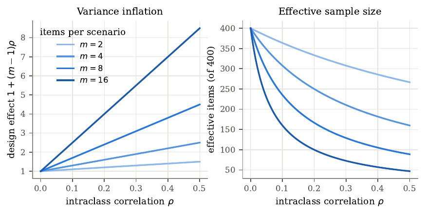
Figure 8. The design effect of clustered items. Left, variance inflation as a function of the intraclass correlation \(\rho\) for different numbers of items per scenario \(m\). Right, the effective number of independent items in a 400-item benchmark. Large scenarios with moderate correlation consume most of the nominal sample size.

In practice cluster sizes are unequal and \(\rho\) is unknown, so the cluster-robust (sandwich) estimator (Liang and Zeger, 1986; Cameron and Miller, 2015) estimates each cluster’s variance directly from its residual total. With \(e_{j} = \bar y_{j} - \hat\mu\) and \(E_{c} = \sum_{j \in c} e_{j}\),

\[\widehat{\Var}_{\text{CR}}(\hat\mu) = \frac{C}{C-1}\cdot\frac{1}{n^2}\sum_{c=1}^{C} E_{c}^2.\]

The factor \(C/(C-1)\) corrects for small samples. The estimator is consistent as the number of clusters grows, whatever the within-cluster structure, and its accuracy depends on the number of clusters, and the number of items leaves it unchanged. With fewer than about 30 clusters it tends to underestimate the variance, and with fewer than about 10 it is unreliable. When every cluster has one item it reduces to the usual independent-items variance, so it is the safe default whenever cluster labels exist. For planning, the analysis-of-variance estimator of \(\rho\) compares the variation of cluster means with the variation within clusters.

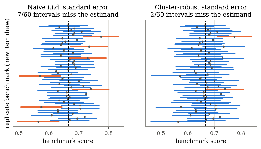
Figure 9. Coverage of 95 percent intervals for clustered items. Each row is a benchmark of 200 items in scenarios of 8, drawn independently from the same generator. The dashed line is the item-population estimand, and intervals that miss it are shown in orange. The naive standard error ignores the shared scenario effect and produces intervals that are too narrow.

Over 400 replicates, the naive interval covers the estimand 90.8 percent of the time and the clustered interval 94.8 percent. The naive interval fails only modestly here because the simulated design effect is moderate; with larger scenarios or stronger shared context the gap widens. The number of independent scenarios, more than the count of items, sets the precision of a clustered benchmark.

Repeated sampling and the variance floor

Sampling a model several times per item reduces the noise from the model’s own randomness, while the noise from which items were chosen stays. With \(K\) samples per item, the law of total variance splits the item mean into

\[\Var(\bar y_{j}) = \Var_{j}(p_{j}) + \mathbb{E}_{j}\!\left[\frac{p_{j}(1-p_{j})}{K}\right].\]

Writing \(\sigma_{b}^2 = \Var_{j}(p_{j})\) for between-item variance and \(\sigma_{w}^2 = \mathbb{E}_{j}[p_{j}(1-p_{j})]\) for mean within-item variance, for \(n\) independent items

\[\operatorname{SE}(\hat\mu) = \sqrt{\frac{\sigma_{b}^2}{n} + \frac{\sigma_{w}^2}{nK}}.\]

Increasing \(K\) shrinks only the second term, and as \(K \to \infty\) the standard error approaches the floor \(\sigma_{b}/\sqrt{n}\), which only more items can lower.

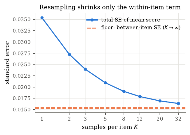
Figure 10. Standard error of the benchmark score as the number of samples per item \(K\) grows, for 200 simulated items. The dashed line is the floor set by between-item variance, which repeated sampling cannot reduce.

You can estimate both components from data with \(K \ge 2\). The unbiased estimate of \(p_{j}(1-p_{j})\) is \(\bar y_{j}(1-\bar y_{j})K/(K-1)\), and averaging it over items estimates \(\sigma_{w}^2\), while the sample variance of the \(\bar y_{j}\) estimates \(\sigma_{b}^2 + \sigma_{w}^2/K\). The ratio \(\sigma_{w}^2/\sigma_{b}^2\) yields a planning rule. Once \(K\) exceeds roughly \(\sigma_{w}^2/\sigma_{b}^2\), the marginal benefit of another sample falls below that of one more item. Greedy decoding removes within-item variance but leaves the model’s uncertainty in place and gives a fixed-item quantity for one configuration, so for capability estimation sampling at the deployment temperature usually teaches more.

Comparing models

Compare two models on the same items, using per-item differences \(d_{j} = \bar y_{Aj} - \bar y_{Bj}\), because pairing removes item-difficulty variance. The variance of the difference is

\[\Var(\hat\delta) = \frac{1}{n}\big[\Var(\bar y_{Aj}) + \Var(\bar y_{Bj}) - 2\Cov(\bar y_{Aj}, \bar y_{Bj})\big].\]

Items hard for model \(A\) tend to be hard for \(B\), so the covariance is positive and subtracting it shrinks the variance. An unpaired analysis omits the covariance and overstates the uncertainty of the difference. With equal item variance \(\sigma^2\) and correlation \(\rho_{\text{pair}}\), the paired variance is \(2\sigma^2(1 - \rho_{\text{pair}})/n\), so at \(\rho_{\text{pair}} = 0.5\) pairing halves the variance. With one sample per item, McNemar’s exact test (McNemar, 1947) uses only the discordant items, since under the null each discordant item is equally likely to favor either model; with clustered items the paired-difference test with cluster-robust standard errors replaces it. A comparison of two models should use the paired difference and set aside any overlap of their separate intervals.

Power and the number of items

Before building a benchmark, compute how many items it needs to detect the smallest difference that would change a decision. Card et al. (2020) showed that many NLP comparisons are underpowered, and the same problem affects biosecurity evaluations. For a two-sided paired test at level \(\alpha\) with power \(1-\beta\), the number of items satisfies \(\delta/\operatorname{SE}(\hat\delta) = z_{1-\alpha/2} + z_{1-\beta}\), and for binary outcomes near base rate \(p\) with pairing correlation \(\rho_{\text{pair}}\) and design effect \(\mathrm{deff}\),

\[n = \frac{\mathrm{deff}\cdot 2p(1-p)(1-\rho_{\text{pair}})\,(z_{1-\alpha/2} + z_{1-\beta})^2}{\delta^2}.\]

This scales as \(1/\delta^2\), so halving the detectable difference quadruples the item count. At \(p = 0.5\) with no pairing benefit and no clustering, detecting a 10-point difference needs 393 items, a 5-point difference needs 1,570, and a 2-point difference needs 9,812.

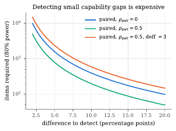
Figure 11. Items required for 80 percent power to detect a difference between two models at \(\alpha = 0.05\), at a base rate of 0.5. Pairing reduces the requirement and clustering increases it. The vertical scale is logarithmic.

Most biosecurity benchmarks have a few hundred items, so they can reliably detect differences of about 10 points and leave 2 or 3 out of reach, and a report that ranks models separated by a few points on such a benchmark is reporting noise. The inverse calculation gives the minimum detectable difference for an existing benchmark,

\[\delta_{\min} = (z_{1-\alpha/2} + z_{1-\beta})\sqrt{\frac{\mathrm{deff}\cdot 2p(1-p)(1-\rho_{\text{pair}})}{n}},\]

which should be reported alongside the benchmark so readers see which comparisons it can support.

The bootstrap and many comparisons

The bootstrap (Efron and Tibshirani, 1993) estimates the sampling distribution of a statistic by resampling, and I turn to it for statistics with no simple variance formula, such as the corrected rate above, and when clusters are too few for the sandwich estimator. The resampling unit must match the dependence structure, so for clustered items you resample whole clusters with replacement and keep all items of a selected cluster together. With very few clusters every bootstrap method becomes unreliable, and the right response is to report that the benchmark has too few independent scenarios.

A typical assessment reports scores for several constructs, models, and conditions, and testing each at \(\alpha = 0.05\) gives a chance of at least one false positive across 20 independent comparisons of \(1 - 0.95^{20} \approx 0.64\). The Holm procedure (Holm, 1979) controls the family-wise error rate, and the Benjamini-Hochberg procedure (Benjamini and Hochberg, 1995) controls the false discovery rate. For safety decisions the asymmetry often runs the other way, since a false negative that misses an actual capability usually costs more than a false positive, so a team may prefer to report uncorrected results and state explicitly how many comparisons it made.

Item response theory refines this. The benchmark score treats every item as equally informative, but items differ. Item response theory (IRT) describes how the probability of a correct answer depends jointly on a respondent’s latent ability and an item’s properties (Lord, 1980; Embretson and Reise, 2000). In biosecurity evaluation it places models and human experts on a common ability scale, identifies which items carry information near a decision threshold, and lets you shorten or adapt a benchmark while holding precision where precision matters. Prior work applied IRT to rank items by informativeness (Rodriguez et al., 2021; Vania et al., 2021) and to estimate full-benchmark scores from small subsets (Polo et al., 2024).

From sum scores to latent ability

The Rasch model (Rasch, 1960) gives each item a difficulty \(b_{j}\) and each respondent an ability \(\theta_{r}\),

\[\Pr(y_{rj} = 1 \mid \theta_{r}) = \sigma(\theta_{r} - b_{j}), \qquad \sigma(x) = \frac{1}{1 + e^{-x}}.\]

When ability equals difficulty the probability of success is one half, and under the Rasch model the raw sum score is a sufficient statistic for ability. Birnbaum (1968) added a discrimination parameter that controls how sharply success rises with ability,

\[\Pr(y_{rj} = 1 \mid \theta_{r}) = \sigma\big(a_{j}(\theta_{r} - b_{j})\big).\]

A negative discrimination, where weaker respondents succeed more often than stronger ones, usually signals a wrong key. On multiple-choice items even a respondent with no knowledge sometimes guesses, so the 3PL model adds a lower asymptote,

\[p_{j}(\theta) = c_{j} + (1 - c_{j})\,\sigma\big(a_{j}(\theta - b_{j})\big).\]

Estimating \(c_{j}\) freely is unstable, so a practical compromise fixes \(c_{j} = 1/k\) for a \(k\)-option item.

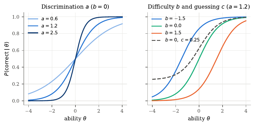
Figure 12. Item characteristic curves. Left, three items with the same difficulty and different discrimination; higher discrimination produces a sharper transition. Right, items of different difficulty, and a four-option item with a guessing floor \(c = 0.25\) (dashed).

In an evaluation the respondents can be models, model configurations, and human experts or novices who took the same items as a baseline, and fitting them together puts them on one ability scale, so “this model’s ability exceeds that of the median expert in the validation pool” has a precise meaning. A single ability dimension assumes the items measure one construct, so using IRT responsibly includes checking fit by construct and by respondent type.

Estimation by joint maximum a posteriori

Given a response matrix \(Y\) with a mask \(M_{rj}\) marking observed responses, the 2PL log-likelihood with a fixed guessing floor is

\[\ell(\theta, a, b) = \sum_{r,j} M_{rj}\Big[ y_{rj}\log p_{rj} + (1 - y_{rj})\log(1 - p_{rj}) \Big],\]

with \(p_{rj} = c_{j} + (1-c_{j})\sigma(z_{rj})\) and \(z_{rj} = a_{j}(\theta_{r} - b_{j})\). Maximizing this directly can diverge, because a respondent who answers everything correctly has maximum-likelihood ability \(+\infty\), so weak priors (\(\theta_{r} \sim \mathcal{N}(0,1)\), \(b_{j} \sim \mathcal{N}(0,2^2)\), \(\log a_{j} \sim \mathcal{N}(0,0.5^2)\)) give a maximum a posteriori estimate instead. The gradient of one term with respect to \(z_{rj}\) is

\[g_{rj} = M_{rj}\left(\frac{y_{rj}}{p_{rj}} - \frac{1 - y_{rj}}{1 - p_{rj}}\right)(1 - c_{j})\,\sigma(z_{rj})\big(1 - \sigma(z_{rj})\big),\]

which reduces to the familiar logistic residual \(M_{rj}(y_{rj} - p_{rj})\) when \(c_{j} = 0\). Summing over the appropriate index and adding the prior terms gives the gradients with respect to \(\theta_{r}\), \(b_{j}\), and \(\log a_{j}\), which L-BFGS uses to fit. Joint estimation treats every ability as a parameter and, with few items per respondent, gives inconsistent item parameters; the standard alternative is marginal maximum likelihood (Bock and Aitkin, 1981). Evaluations often reverse the educational-testing setting, with many items and a few dozen respondents, where joint MAP with weak priors is adequate and much simpler. The 2PL needs constraints for identification, so you standardize abilities to mean zero and unit variance and transform item parameters to match, and because this fixes the scale relative to the fitted sample, a later fit with a new, stronger model shifts the scale unless secure anchor items hold it fixed.

Fisher information and targeted testing

An item is most informative about respondents whose ability is near its difficulty, and information adds across items, so you can build a test to be precise where a decision is made. For a Bernoulli outcome with success probability \(p(\theta)\), the Fisher information is

\[I(\theta) = \frac{[p'(\theta)]^2}{p(\theta)\big(1 - p(\theta)\big)},\]

which for the 3PL model becomes

\[I_{j}(\theta) = a_{j}^2\,\frac{(p_{j} - c_{j})^2}{(1 - c_{j})^2}\,\frac{1 - p_{j}}{p_{j}}.\]

For the 2PL case this is \(a_{j}^2\,p_{j}(1 - p_{j})\), which peaks at \(\theta = b_{j}\) with height \(a_{j}^2/4\); a guessing floor lowers the information and shifts its peak slightly above \(b_{j}\). Test information is \(I(\theta) = \sum_{j} I_{j}(\theta)\), and the standard error of an ability estimate is approximately \(1/\sqrt{I(\theta)}\).

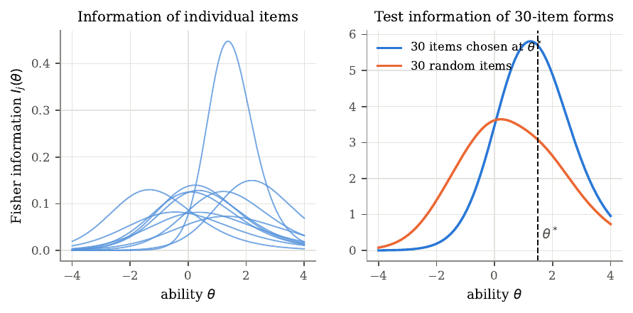
Figure 13. Fisher information. Left, information curves of a sample of items from a 120-item pool. Right, test information of a 30-item form built from the items most informative at a decision threshold \(\theta^* = 1.5\), compared with a random 30-item form. The targeted form concentrates precision where the decision is made.

At the threshold the targeted form has 1.85 times the information of the random form (5.69 against 3.07), so its ability standard error there is about 27 percent smaller. Before trusting IRT estimates I run a recovery study at the data’s size.

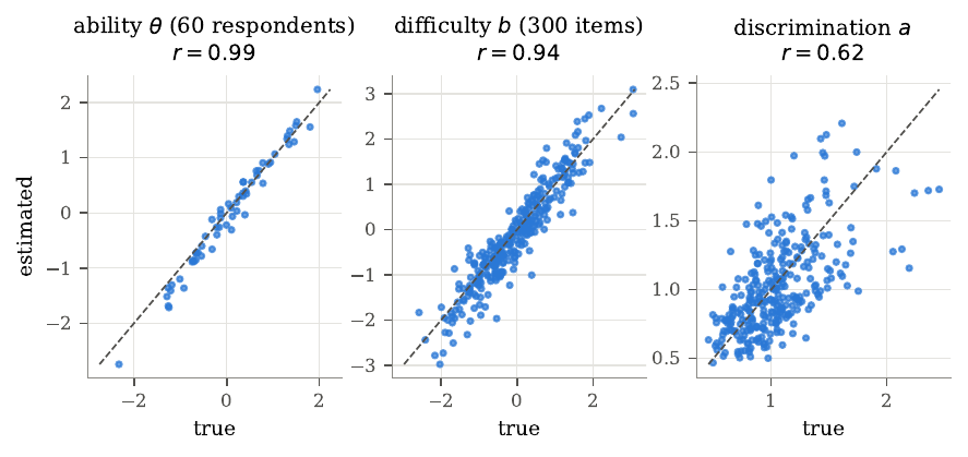
Figure 14. Recovery of 2PL parameters by joint MAP estimation from a simulated 60-respondent, 300-item response matrix. Dashed lines mark perfect recovery. Abilities and difficulties recover well, with correlations 0.99 and 0.94. Discriminations, each estimated from only 60 responses, recover less precisely, at correlation 0.62.

Because discrimination recovers weakly with few respondents, analysts should confirm stability across refits before basing any decision on individual item discriminations, such as dropping items for low discrimination. A safety decision asks whether ability exceeds a threshold, and once a calibration study has fixed the item parameters, you can place a new model on the scale with the expected a posteriori estimate, the posterior mean of \(\theta\) over a grid,

\[\hat\theta_{\text{EAP}} = \frac{\int \theta\, L(y \mid \theta)\,\phi(\theta)\,d\theta}{\int L(y \mid \theta)\,\phi(\theta)\,d\theta}.\]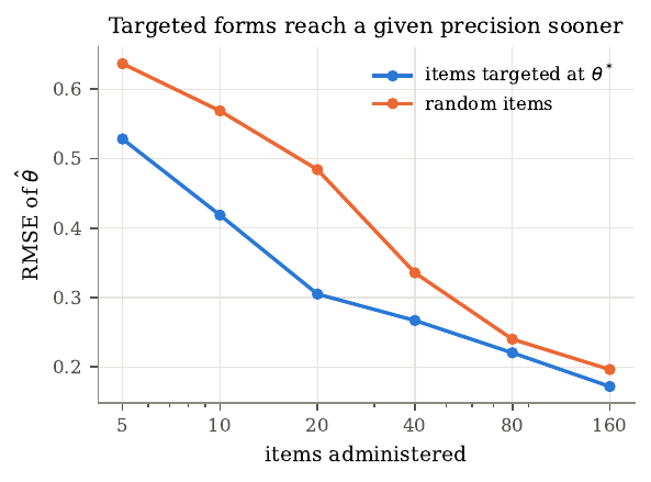

Figure 15. Error of the ability estimate for a respondent at the threshold, as a function of the number of administered items. Forms built from items targeted at the threshold reach a given precision with fewer items than random forms. Each point averages 60 simulated respondents.

With 20 targeted items the root-mean-square error is 0.30, while 40 random items give 0.34, so the random form needs more than twice as many items to match the targeted one. Fully adaptive testing goes further, picking each next item from the current estimate (van der Linden and Glas, 2010), which resolves a model clearly far from the threshold with few items and spends the remaining budget where decisions are hardest. Targeted forms carry a security cost, since known items can be trained on and a small targeted form is easier to compromise, so item pools should be large, rotate, and be held at the tier of their most sensitive items. When models and humans share one scale, two cautions apply. The validation expert pool is usually small and may fall short of the threat model’s actor population, and a model may exceed experts on recall of written knowledge while falling far short on hands-on skill, so a shared scale makes sense only for a construct on which both groups use the same capability.

Agentic and multi-attempt evaluations

Single-turn questions measure what a model knows and can state, but many capabilities in a threat model involve sequences of actions, such as searching the literature, writing and running code, noticing an error, and trying again. Agentic evaluations place the model in an environment with tools and ask it to complete a multi-step task (Kinniment et al., 2023; Phuong et al., 2024). Open-source tooling such as Inspect (UK AI Safety Institute, 2024) provides the components. Three properties of the environment matter. Realism, since the tools should match the elicitation set of the threat model; determinism and logging, since runs vary and every tool call and result should be logged with timestamps; and containment. Agentic biosecurity evaluations must keep the model walled off from anything that acts in the physical world or that could place an order, send a message to a third party, or retrieve restricted material from outside the evaluation. Tools should run in a sandbox with no network access by default, read-only mounts, a non-root user with capabilities dropped, quotas, and a host-enforced deadline, with network access allowed only to an allowlist where realism requires it and every request logged. You measure capability by scoring outputs inside the sandbox, with the model kept from acting.

Counting repeated attempts

An actor can try a task many times. If a model succeeds with probability \(p\) per independent attempt, the probability that at least one of \(k\) attempts succeeds is

\[\text{pass@}k = 1 - (1 - p)^k.\]

A model that succeeds 10 percent of the time per attempt succeeds at least once in 10 attempts with probability 0.65 and in 32 with probability 0.97, so a low per-attempt rate still carries risk when an actor can try many times and recognize success. I keep coming back to how fast a 10 percent per-attempt rate compounds, reaching 0.97 by 32 tries. In practice \(p\) is unknown, and from \(n \ge k\) samples with \(c\) successes the plug-in estimate \(1 - (1 - c/n)^k\) is biased downward by Jensen’s inequality. Chen et al. (2021) derived an unbiased estimator,

\[\widehat{\text{pass@}k} = 1 - \frac{\binom{n - c}{k}}{\binom{n}{k}},\]

which equals the probability that a random \(k\)-subset of the \(n\) outcomes contains a success; averaging over the i.i.d. outcomes gives \(1 - (1-p)^k\). Computed as a stable product, with true per-attempt rate 0.15, \(n = 20\), and \(k = 5\), its mean over 20,000 replicates is 0.558 against the true 0.556. Some threat models instead need every attempt to succeed, for which the unbiased estimator of pass\(^k\) is \(\binom{c}{k}/\binom{n}{k}\).

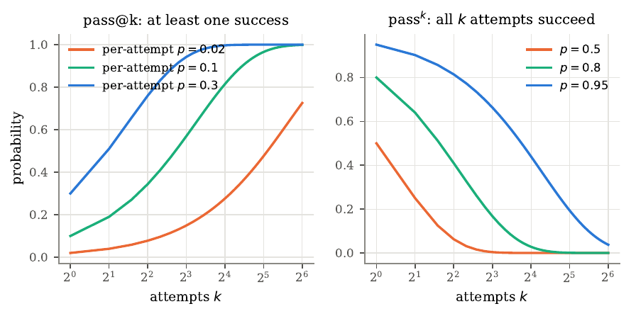
Figure 16. Repeated attempts. Left, probability of at least one success in \(k\) attempts (pass@\(k\)) for three per-attempt rates. Right, probability that all \(k\) attempts succeed (pass\(^k\)); a model with per-attempt success 0.8 completes 8 consecutive attempts with probability 0.17. Which quantity matters depends on whether the actor in the threat model can recognize success.

pass@\(k\) assumes the actor can tell which attempt succeeded, which unit tests provide in coding, while a written protocol often requires carrying it out. If the actor’s imperfect check accepts a correct attempt with probability \(t\) and an incorrect one with probability \(f\) and takes the first accepted attempt, the expected success rate lies between the single-attempt rate and pass@\(n\). I call the gap between pass@\(n\) and this verified rate the oracle gap. Reporting pass@\(k\) alone assumes a perfect verifier and overstates what most actual actors could achieve, while reporting only the single-attempt rate assumes no verifier and understates it. A threat model should state what verification the actor population has, and the evaluation should report the corresponding quantity.

Time horizons

Agentic tasks vary greatly in length, and Kwa et al. (2025) proposed summarizing a suite by the task length at which a model succeeds half the time, where length is the time a skilled human takes. Modeling success as a logistic function of log task length,

\[\Pr(\text{success on } t) = \sigma\big(\beta(\log_{2} h_{50} - \log_{2} \ell_{t})\big),\]

gives the 50 percent time horizon \(h_{50}\) and a slope \(\beta\), and the horizon at any other success level \(q\) is \(h_{q} = h_{50} \cdot 2^{-\operatorname{logit}(q)/\beta}\).

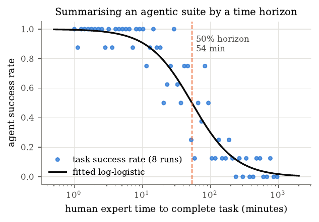
Figure 17. Time-horizon summary of an agentic suite. Each point is a task, placed by the time a skilled human needs and the fraction of 8 agent runs that succeeded. The curve is the fitted log-logistic model, and the dashed line marks the estimated 50 percent horizon.

Fitting 60 simulated tasks from 1 to 960 minutes with a true horizon of 45 minutes gives an estimate of 54 minutes with a bootstrap interval of 43 to 66 minutes, which contains the truth; horizon estimates from a few dozen tasks are uncertain by a factor of about 1.5 in each direction. Two limitations matter for biosecurity. The horizon depends on the task distribution, so a software horizon applies to software and stops short of laboratory planning, and the human completion time is itself an estimate, whose error attenuates the fitted slope and adds uncertainty beyond what the task bootstrap captures.

Elicitation

A capability evaluation that uses weak elicitation measures the evaluator’s effort as much as the model, and the capability estimand is a maximum over elicitation methods. Davidson et al. (2023) found that post-training enhancements can raise performance substantially while the base model stays as is, so a score under default prompting is a lower bound and possibly a loose one. Searching over elicitation conditions and reporting the best one pays a statistical cost. If every condition has the same true score \(p\), the maximum of several noisy scores is biased upward, because the maximum selects the condition whose noise happened to be most positive, the winner’s curse. This is the same selection-on-error mechanism that opened the guide, now acting on elicitation conditions in place of candidate designs.

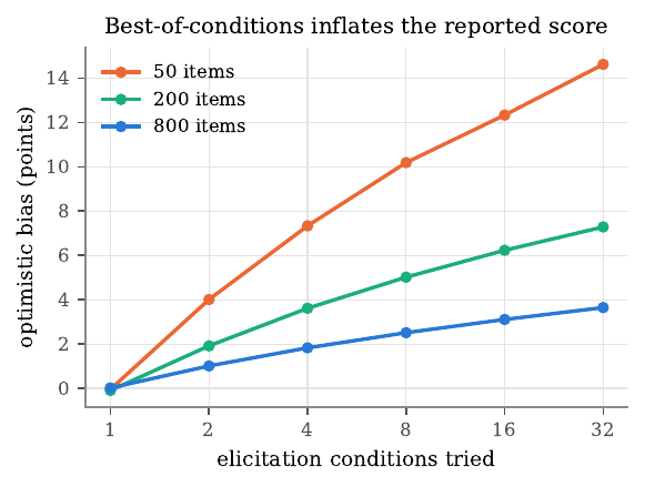
Figure 18. Optimistic bias from reporting the best of several elicitation conditions with equal true scores of 0.5, as a function of the number of conditions tried and the benchmark size.

On a 100-item benchmark, the best of 4 equally capable conditions overstates the true score by 5 points on average, and the best of 16 by 9 points; since actual conditions evaluated on the same items are positively correlated, this is an upper bound. The standard remedy is a held-out split, developing elicitation on one set of items and evaluating the chosen configuration once on a separate set, split by cluster so no scenario straddles both halves. In safety evaluation the winner’s curse biases the capability estimate upward, which is the conservative direction for a rule-out decision, so some teams accept it deliberately, but even then they should report its size, because a large upward bias can trigger safeguards on noise and distort comparisons across generations that tried different numbers of conditions.

Sandbagging and evaluation awareness

A capability evaluation assumes the model tries its best, and this can fail. Van der Weij et al. (2024) showed that models can be prompted or fine-tuned to underperform selectively on dangerous-capability evaluations while performing normally elsewhere, called sandbagging, and Greenblatt et al. (2024) studied password-locked models whose hidden capability fine-tuning often recovers. Related work shows models can tell when they are being evaluated (Laine et al., 2024) and can act differently when they believe they are being tested or trained (Greenblatt et al., 2024; Meinke et al., 2024; Hubinger et al., 2024). A low score therefore has two explanations. The model lacks the capability, or it has the capability and withholds it. Fine-tuning on related demonstrations tests whether a capability is latent, which only parties holding the weights can run, on helpful-only checkpoints inside the secure environment. External evaluators rely on matched benign controls and on person-fit statistics, which flag respondents who fail easy items while passing hard ones. Each of these checks is suggestive, and reports should state which ones the team ran.

Case study, when the evaluator is the attack surface

The containment and logging rules above protect the environment, but in a full agent loop the evaluator itself is a component, and a component can be gamed. I red-teamed a verifier, the part that decides which of an agent’s proposals to keep, in a setting where ground truth exists so I can measure the actual quality of what it keeps. A fully leaked scorer reached an AUROC of 0.991 and added only 0.028 good candidates per batch over random, against 1.082 for a truthful scorer. Worse, a probe that spot-checks a quarter of decisions detects 99.2 percent of attacks and recovers only about 10 percent of the lost value when its fallback is random selection, so catching an attack and undoing it are different things. Getting to 17 percent needs a second source of capability beyond the attacker’s control, a model trained on the campaign’s own measurements, which is a different fix from the detector.

This is the same audit-sweep result named earlier, and the lesson for an agentic evaluation is that detection and recovery are different quantities. A verifier that clears a trust gate on discrimination (AUROC 0.991) can still add nothing to the value of what it keeps, so an agentic harness that scores a model through a verifier has to measure the realized quality of the kept outputs against ground truth, beyond the verifier’s discrimination.

Contamination, saturation, and sensitivity

The earlier methods assume a benchmark score reflects the model’s ability on the construct, and three common problems break this assumption. Contamination occurs when items or their answers appear in training data, so the score measures recall. Saturation occurs when strong models approach the benchmark’s ceiling, so further capability gains stop showing. Design sensitivity occurs when arbitrary choices, such as the prompt template, move the score as much as the differences you are studying.

Canaries and n-gram overlap

Keeping items out of training data prevents contamination more reliably than any later test can detect it. A canary string is a unique random string placed in every file that contains items, which BIG-bench introduced and asked developers to filter out (Srivastava et al., 2023). A model that can complete the canary from its first half has very likely trained on files that contained it, so a positive canary test is strong evidence of exposure, while a negative test is weak evidence of a clean model, since items can leak apart from their canary. Developers with training-data access can search directly for long shared word sequences, since a 13-word sequence shared between an item and a training document is unlikely by chance, though n-gram overlap misses paraphrased leaks. To catch those, Golchin and Surdeanu (2024) prompt a model with the beginning of an item and the name of its source benchmark and measure whether it reproduces the rest more closely than chance; because these methods run the model on item content, you must run restricted items inside the secure environment.

Temporal splits and perturbation tests

When training data are unavailable, two statistical tests detect contamination from scores alone. Items written after a model’s training cutoff lie outside its training data, so if the model scores much higher on items written before the cutoff, and difficulty does not explain it, memorization is a likely explanation.

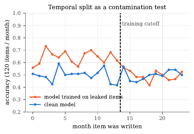
Figure 19. Temporal split as a contamination test. Monthly accuracy on items grouped by the month they were written. A model trained on leaked items (orange) scores higher only on items written before its training cutoff (dashed line); a clean model (blue) shows no change at the cutoff.

In the simulation a model trained on leaked items scores about 15 points higher before its cutoff and falls to the clean model’s level afterward. The test is only as good as the comparison, since if item style or difficulty drifted over time the pre and post groups differ for unrelated reasons, so you compare the suspect model’s pre-post gap with that of a model whose cutoff postdates all items, because drift affects both while contamination affects only one. A second test rewrites each item so its meaning and answer stay fixed while its surface form changes; a model that reasons scores about the same, while a model that memorized the original text loses accuracy. Since original and perturbed versions share an item, the comparison is paired. Option reordering is the cheapest perturbation and needs no review, which is one reason the harness shuffles options by default.

Saturation and the label-noise ceiling

A benchmark stops discriminating between models before scores reach 100 percent, and answer-key errors make saturation arrive early (Ott et al., 2022). Let \(\kappa_{j}\) be the probability that item \(j\)’s key is correct. A perfect respondent matches the key on items with correct keys and, for a four-option item with a wrong key, matches with probability near zero, so the maximum attainable expected score is approximately

\[\mu_{\max} \approx \frac{1}{n}\sum_{j} \kappa_{j}.\]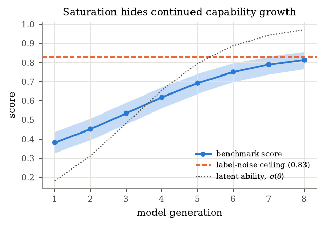

Figure 20. Saturation. Simulated benchmark scores (with 95 percent Wilson bands) for eight model generations of steadily increasing latent ability (dotted). Because 17 percent of answer keys are wrong, scores approach a ceiling of 0.83 (dashed) and stop tracking the continued growth in ability.

The last few generations fall within one another’s confidence intervals even though their abilities differ substantially, so an observer who looked only at the scores would conclude progress had stopped. Three responses help. Clean the answer keys, since items where several strong models agree with each other and disagree with the key are good candidates for review; add harder items, guided by where the IRT pool has little information; and retire a saturated benchmark from decision-making while still reporting it for continuity.

Sensitivity to evaluation design

Language-model scores are sensitive to choices that should not matter. Sclar et al. (2024) found that prompt-formatting changes can move accuracy by tens of points, Madaan et al. (2024) measured variance across seeds large enough to change rankings, and Biderman et al. (2024) documented how implementation details produce irreproducible results. A factorial design over a few levels of each factor decomposes the variance of the resulting scores, with the share due to factor \(f\) being the variance of its level means around the grand mean, divided by the total variance.

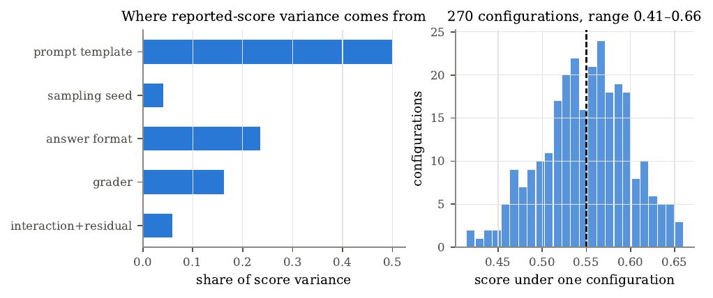
Figure 21. Sensitivity of a score to evaluation design. Left, share of variance in a simulated model’s score attributable to each design factor in a full factorial over 270 configurations. Right, distribution of the score across configurations; the dashed line is the true mean.

In the example, scores range from 0.41 to 0.66 for a single model whose average is 0.55. Prompt template accounts for half of the variance, answer format for 24 percent, grader for 16 percent, and sampling seed for 4 percent. An evaluation that reported one configuration could have reported any value in that range, and two models whose single-configuration scores differ by 10 points could easily be equally capable. The remedy has two parts. Standardize and document the factors that matter and run each evaluation under several levels of each, so the reported score averages over reasonable choices, and compare models under the same configurations so design effects cancel in the paired difference.

Case study, a genomic model and protein function

So far I have treated validity, held-out transfer, and confound controls in the abstract. The next two case studies run them in full on live models, starting with a transfer question that a single control settles. I built biologos to ask whether a model trained on DNA knows anything about protein function, measured against a protein model on the same 25 deep mutational scanning assays. DNA and protein are two encodings of one molecule related by a map that is known, which makes biology a clean place to ask a transfer question the rest of machine learning can only ask loosely. The measurement uses deep mutational scanning assays, which measure the fitness effect of many single mutations to a protein. I matched every scorer on the same 25 assays and measured the Spearman correlation between the scorer and the measured effects, so a genomic model, a protein model, a substitution matrix, and a few chemical properties all answer the same question on the same data.

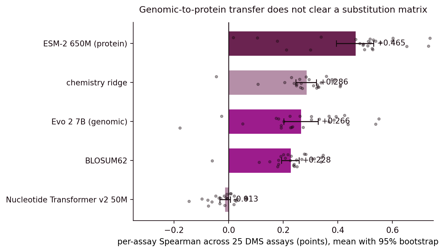
Figure 22. Mean Spearman across the 25 assays, with 95 percent intervals. ESM-2 650M, a protein model, reaches 0.4655. A chemistry ridge fit leave-one-cluster-out reaches 0.2860. Evo 2 7B, a genomic model, reaches 0.2658. BLOSUM62 alone reaches 0.2282. The Nucleotide Transformer v2 50M sits at minus 0.0132.

The comparison that matters is Evo 2 against the substitution matrix. I ran all four scorers on the same 25 assays, and the genomic model lands close to a plain substitution matrix. Evo 2 minus BLOSUM62 is plus 0.0376, in an interval of minus 0.012 to plus 0.087 that contains zero, and Evo 2 is higher in 14 of the 25 assays, so the data do not distinguish the two at this sample size, a test that would have missed even a matrix 37 percent better. Against a set of supervised chemical features, fit leave-one-cluster-out, Evo 2 is behind at minus 0.0202, in an interval of minus 0.0729 to plus 0.0354 that contains zero and higher in 9 of the 25 assays, and that comparison differs in kind because the chemistry ridge is supervised while Evo 2 is scored zero-shot.

So a genomic model at Evo 2 scale does acquire protein-fitness signal, and the careful way to state it is that the signal is not distinguishable from a substitution matrix at this sample size, is behind a set of supervised chemical features in an interval that contains zero, and sits far below a protein model. The Nucleotide Transformer family carries no signal at all at any scale I tested, and its scaling trend falls short of Evo 2, because extrapolated to 7B it predicts plus 0.028 against the plus 0.266 measured, short by a factor of 9.5.

Four things I got wrong first

The corrections are the point, so I list them before anyone leans on the headline.

I retracted a reading-frame result. A genomic model appeared to confuse a gene with the same gene read one nucleotide out of frame, but the frameshift was a rotation, which apart from one wrap junction is actual genomic sequence read one base later. Once I rank the four conditions by whether they produce an actual genomic string, the whole table reproduces with no appeal to reading frame.

I falsified a representation-transfer claim with its own control. A probe on genomic embeddings scored plus 0.141 on unseen residues, which read as weak transfer, and then it scored plus 0.143 after frameshifting and plus 0.129 on the reverse complement. A representation invariant to destroying the reading frame sits below the protein level, because under any encoding the codon determines the amino acid, so the nucleotides at a varying site already are residue identity.

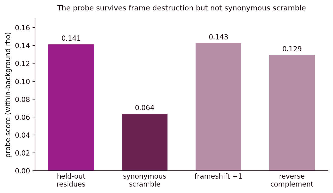
Figure 23. The transfer probe scores about the same on held-out residues, 0.141, on frameshifted input, 0.143, and on the reverse complement, 0.129, so it is invariant to destroying the reading frame. It drops only under a synonymous scramble, 0.064, which changes codons while leaving amino acids fixed, so the probe is reading codon identity, which determines the amino acid, short of protein-level structure.

I found a context dose-response that was measuring composition. Actual genomic context made one model monotonically worse, with a trend of minus 0.771, and composition-matched shuffled flanks that carry no genomic information reproduce it at minus 0.633. A second model with a wider window produced a clean positive trend that its shuffled twins fully account for, so context trends on this landscape run in both directions from noise.

I made a general claim that was too general. “A genomic model carries no protein-fitness signal” held for the Nucleotide Transformer family, and I wrote it as though it held for genomic models, and Evo 2 refutes it. The corrected claim is the one above. At Evo 2 scale the signal exists and does not clear a substitution matrix. biologos is independent research, a measurement of transfer in place of a bid to build a better model. The code is at github.com/saanviiyer/biologos.

Case study, signature steering in a protein model

This second case study is the full lab report behind the confound and held-out-transfer tests, how the PRISM pipeline works, what each control measures, and which file each number comes from. It is the methods record behind its companion essay The probe works and the understanding is not there.

The pipeline

A mutational signature is the characteristic pattern of DNA base substitutions a mutational process leaves behind, and the COSMIC catalog lists 78 single-base-substitution signatures, each a probability distribution over base changes in its trinucleotide context. PRISM asks whether those processes move the proteins they alter toward particular regions of a protein model’s representation.

For each signature, the operator walks a coding sequence and samples substitutions from that signature’s channel weights for the local trinucleotide. It writes edits in place, so a substitution can change the context for the next position, which is rare at per-position probabilities of order ten to the minus two. The current configuration generates ten mutants per protein and signature condition. The pipeline omits reverse-complement substitutions.

The source proteins come from two Pfam clans. There are 65 usable accessions across 12 families in CL0023, the P-loop NTPase clan, and 9 accessions from a single family in CL0072. Other clan runs exist in the archive, so the two-clan framing is a selection from more runs, which I state plainly below.

The pipeline translates and embeds each mutant with ESM-2 8M. Mean pooling over residue vectors, excluding the start and end tokens, gives one vector per protein. Displacement toward a Pfam family is the signed change in cosine distance to that family’s centroid, so a positive value means the mutant mean sits closer to the family than the wild type does. The centroid library holds 27,481 Pfam family centroids at 320 dimensions. Steering analyses use hidden layer 5 of the same model.

Two notes on the model size, because they bound what the pipeline can say. The trajectory work runs on ESM-2 8M, with the 650M model left aside. A 650M centroid library exists but covers only 492 clan-restricted families, which falls short of a catalogue-wide comparison, so these results stay untested at a larger model scale.

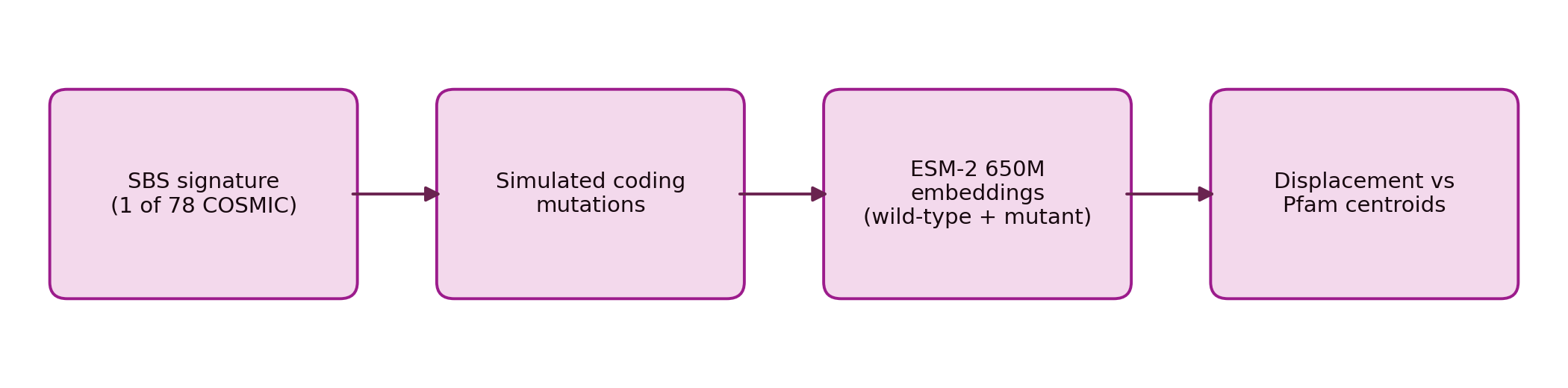
Figure 24. The pipeline runs from an SBS signature, to simulated coding mutations, to ESM-2 embeddings of wild-type and mutant proteins, to displacement measured against Pfam centroids.

SBS17a ranks first toward PF17041 in both clans

On the raw geometry, SBS17a is the top-ranked signature of 78 for directing sequences toward the Pfam family PF17041, and it holds that rank in both CL0023 and CL0072. I found SBS17a at the top of all 78 signatures toward PF17041, and it held in both clans. The same direction in two protein contexts is what an actual effect would produce.

The corrected rerun changes how much that recurrence is worth. The legacy pipeline translated each mutant to the first stop codon. Mapping stop codons to X and continuing translation removes nearly all of the between-signature length variance, and SBS17a stays first in both clans, with concentration rising from 31.6% to 71.7% in CL0023 and from 68.3% to 100.0% in CL0072. But PF17041 attracts more signatures under read-through, CL0072 hubness rises from 1.13% to 5.35%, and enrichment falls from 60.7 times to 18.7 times. Six signatures select PF17041 as their modal CL0072 target, and other pairs also reach 100% concentration. The rerun keeps the association and removes the earlier claim that SBS17a was unique in it.

One more bound on this arm. The PF17041 centroid is built from four seed sequences.

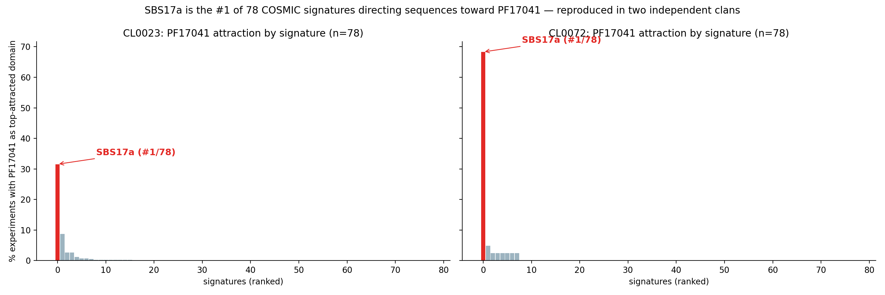
Figure 25. SBS17a is the top-ranked signature of 78 for directing sequences toward PF17041 in both clans. The bar heights are the pre-read-through concentrations, 31.6% in CL0023 and 68.3% in CL0072, which the read-through rerun raises to 71.7% and 100% while keeping SBS17a first.

Length explains most of the displacement magnitude

Premature stops tie signature identity to protein length. Signatures differ in stop-codon probability, and mean-pooled embeddings depend on the translated sequence, so length offers an explanation for displacement that needs no functional shift.

Fitting mean absolute displacement on log translated length, one point per signature across all 78, gives R-squared 0.941 within CL0023. Length alone accounts for 0.941 of the variance in displacement. That is an ordinary least-squares fit on log length, and the fraction of variance it accounts for describes a per-signature summary. Per-protein movement lies outside it. Two provenance notes matter here. The original analysis reported R-squared 0.925 for the same relationship, and I found no code or saved output that produces it. The archived re-derivation that gives 0.941 used 68 source sequences where the retained trajectory panel has 65, so it re-analyzes a slightly different panel. The pairwise arm shows a weaker length association at R-squared 0.53.

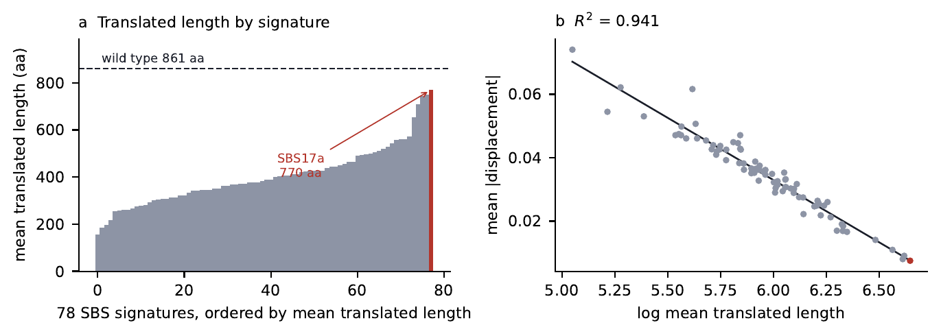
Figure 26. Signatures differ in how long their translated sequences are, because they differ in stop-codon probability, and mean absolute displacement falls almost perfectly with log translated length at R-squared 0.941 across the 78 signatures.

A composition-matched scramble reproduces 72% of the steering, on one readout

The steering arm adds a norm-matched direction vector at hidden layer 5 to held-out wild-type embeddings and measures how far that moves them toward the PF17041 centroid. The measured SBS17a direction reduces cosine distance by 0.0425. A context-scrambled direction, which preserves composition and destroys the signature’s trinucleotide structure, reduces it by 0.0306. The ratio is 72% over five seeds, which is why I read this effect as predominantly compositional.

That 72% belongs to that readout and holds there alone. On the trajectory readout the same scramble control retains only about 34% of the excess above uniform, with measured, scrambled and uniform concentrations at 0.4923, 0.1900 and 0.0360. Two controls of the same name give different answers depending on what they are measuring, so I report the readout alongside the ratio.

A composition follow-up narrows this further. Amino-acid frequencies alone predict cosine distance to the PF17041 centroid at grouped cross-validated R-squared 0.339. On the change in distance, that falls to 0.0966, so composition explains about a tenth of the movement itself. The closed-loop design arm found signature-guided minus composition-matched at -0.0027, p = 0.875.

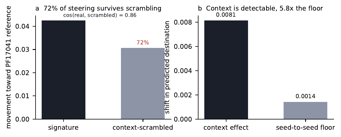
Figure 27. The measured SBS17a direction reduces cosine distance to the PF17041 centroid by 0.0425, and a context-scrambled direction that preserves composition keeps 72% of that movement. The right panel shows the context effect, 0.0081, sitting 5.8 times above the seed-to-seed floor of 0.0014.

The recommender, two evaluations, not one

The inverse-design recommender ranks signatures for a requested Pfam-to-Pfam transition. A random forest reads the origin centroid, the target centroid, their difference, and each signature’s 96-channel COSMIC profile, over 35,403 positive-attraction transitions spanning 75 proteins.

It gets scored two ways, and the two are different tasks. The archived in-distribution run reports AUC 0.94, a binary discrimination between a measured transition and sampled negative signatures on a protein-grouped split. The leave-signatures-out run is a 78-way identification with whole signatures held out as both positives and negatives across five folds, and there top-1 accuracy is 0.775% and top-5 is 7.125%. I ran the leave-signatures-out split, and top-1 came in below a uniform guess. Top-1 sits below the 1.28% a uniform guess over 78 classes would give. With SBS17a excluded from training, the model ranks it first in none of 158 test cases. A separate archived run gives top-1 0.725% and top-5 7.975%, which is the source of an earlier 0.7% in my own prose. The canonical values are the 0.775% ones.

AUC measures discrimination over score thresholds on familiar mechanisms. Top-k measures whether the right signature surfaces for a mechanism held out of training. Reporting only the first would make a recommender that fails out of distribution look like one that works.

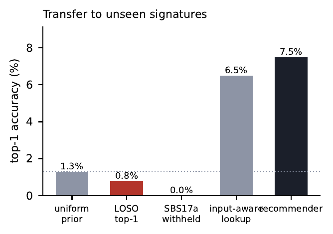
Figure 28. Transfer to unseen signatures. Leave-signatures-out top-1 accuracy is 0.775%, plotted rounded to 0.8%, below the 1.28% a uniform guess over 78 classes would give, and 0.0% when SBS17a itself is withheld.

What is not in PRISM

PRISM measures geometry inside a protein model’s representation, so every number above is a statement about the model. It does not establish biological function. SBS17a is not a validated functional driver on this evidence. The length relationship accounts for most of the displacement magnitude, and the scramble control takes most of the steering. The read-through rerun removes the uniqueness claim, and the recommender does not transfer to held-out mechanisms. There is no residue-level attribution. Nothing here isolates which positions carry whatever signature-specific residual survives the composition and length controls, and that is the experiment this work points at next.

Human uplift trials

Capability and propensity evaluations run the model alone. Uplift concerns how much the model adds to what a human can do, and because it is a causal effect, a randomized controlled trial is the design that estimates it with the fewest assumptions. I adapt clinical-trial methodology (Schulz et al., 2010; Jennison and Turnbull, 2000) and published uplift studies (Mouton et al., 2024; Patwardhan et al., 2024), and borrow from randomized studies of AI assistance for developers (Peng et al., 2023) and consultants (Dell’Acqua et al., 2023).

Why randomize, and how to design

An observational comparison between people who chose the model and people who declined it confounds model access with everything that drives the choice. Random assignment breaks this link, so the expected difference in outcomes between arms equals the average causal effect in the participant population. Randomization guarantees comparability only in expectation, so covariate adjustment and stratified randomization reduce chance imbalance in baseline skill.

The minimal design has two arms. The control arm receives the resources the threat model assumes an actor has apart from the model, typically internet access and standard references, and the treatment arm receives the same plus the model. The participant population should match the actor population as closely as ethics and security allow, with a baseline skill measure collected before randomization to support both stratification and adjustment. For ethical and security reasons trials use proxy tasks, either written planning tasks that graders score but no one carries out, or tasks from benign areas of biology that need the same skills, and the trial’s validity depends on how well those proxies represent the actual steps. The team should specify the primary outcome, often binary task success against a rubric with critical criteria, before the trial, and graders should be blind to arm, which requires removing any trace of model use from the submitted work.

Sample size

Uplift trials are expensive per participant, so they are often too small, and a trial too small to detect a decision-relevant effect leaves the claim of an absent effect unsupported. For a binary outcome with success probabilities \(p_{0}\) and \(p_{1}\) and \(n\) participants per arm, with pooled rate \(\bar p = (p_{0} + p_{1})/2\),

\[n = \frac{\Big[z_{1-\alpha/2}\sqrt{2\bar p(1-\bar p)} + z_{1-\beta}\sqrt{p_{0}(1-p_{0}) + p_{1}(1-p_{1})}\Big]^2}{(p_{1} - p_{0})^2}.\]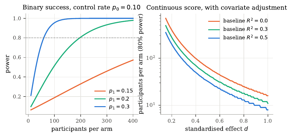

Figure 29. Power of uplift trials. Left, power to detect an increase from a control success rate of 0.10 to three treatment rates, as a function of participants per arm; the dashed line marks 80 percent power. Right, participants per arm needed for 80 percent power on a continuous outcome, as a function of the standardized effect, with and without adjustment for a baseline covariate that explains a fraction \(R^2\) of outcome variance.

To detect an increase from 10 percent to 25 percent at 80 percent power needs 100 participants per arm, and in 1,000 simulated trials the Newcombe interval excluded zero 82.1 percent of the time. An increase from 10 to 15 percent needs several hundred per arm, and a trial with 50 per arm and a control rate of 10 percent has 80 percent power only for increases of 22 points or more. For a continuous outcome with standardized effect \(d\),

\[n = \frac{2(z_{1-\alpha/2} + z_{1-\beta})^2}{d^2},\]

so at 80 percent power \(d = 0.2\) needs 393 per arm, \(d = 0.5\) needs 63, and \(d = 0.8\) needs 25. A baseline covariate that explains a fraction \(R^2\) of outcome variance reduces the required sample to \((1 - R^2)n\), which is usually the cheapest way to increase power. When participants are nested in groups or work in teams, the design effect applies and the unit of analysis becomes the group, which makes team-based trials much more expensive.

Analysis and covariate adjustment

The primary estimate for a binary outcome is the risk difference \(\hat p_{1} - \hat p_{0}\), whose interval needs a method beyond the Wald formula. Newcombe (1998) recommended a hybrid combining the Wilson intervals of the two arms; with \([l_{0}, u_{0}]\) and \([l_{1}, u_{1}]\) the Wilson intervals, the interval for \(p_{1} - p_{0}\) is

\[\left[\hat\delta - \sqrt{(\hat p_{1} - l_{1})^2 + (u_{0} - \hat p_{0})^2},\;\; \hat\delta + \sqrt{(u_{1} - \hat p_{1})^2 + (\hat p_{0} - l_{0})^2}\right].\]

Adjusting for a prognostic baseline covariate increases power while leaving the treatment effect unbiased, and for binary outcomes analyzed with logistic regression it also changes which effect is estimated. Fitting \(\operatorname{logit}\Pr(Z_{i} = 1) = \beta_{0} + \beta_{1}\,\text{arm}_{i} + \beta_{2}\,x_{i}\) by Newton-Raphson, the arm coefficient is the log odds ratio among participants with the same baseline skill. In simulated trials with 120 per arm, a control rate of 0.2, and a true conditional odds ratio of 2, the unadjusted analysis detected the effect in 50.9 percent of trials and the adjusted in 58.4 percent. Part of the gain is variance reduction, and part is non-collapsibility. In logistic regression the conditional odds ratio is farther from 1 than the marginal one even when skill is perfectly balanced (Gail et al., 1984), so the unadjusted and adjusted analyses estimate different quantities. The unadjusted estimates the marginal effect (“how much does model access change the success rate in this population?”) and the adjusted the conditional effect (“for a participant of given skill?”). For uplift claims the marginal risk difference is usually most interpretable, and standardization recovers it from the adjusted model (Kahan et al., 2014).

Demonstrating the absence of uplift

A non-significant result leaves the absence of uplift unproven, because a small trial retains the null for most true effects, large ones included. To support a claim of no meaningful uplift, a trial must show the effect is smaller than a pre-specified margin \(\Delta\), the largest effect that would count as negligible. The two one-sided tests procedure (TOST) tests \(H_{01}\colon \delta \le -\Delta\) and \(H_{02}\colon \delta \ge \Delta\) (Schuirmann, 1987; Lakens, 2017), and rejecting both at level \(\alpha\) supports \(-\Delta < \delta < \Delta\), which is equivalent to the \((1 - 2\alpha)\) confidence interval lying entirely inside the band.

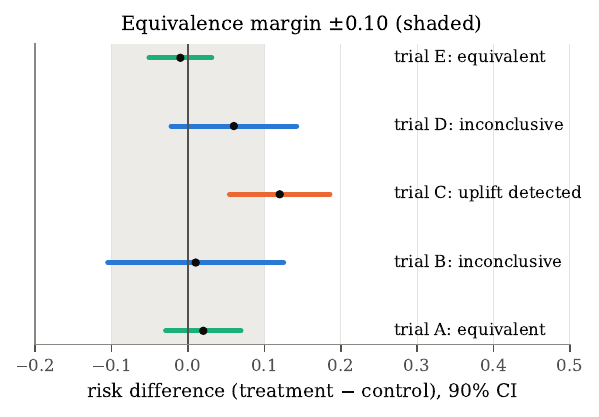
Figure 30. Equivalence testing. Five hypothetical trials, each shown as a 90 percent interval for the risk difference. The shaded band is the equivalence margin of \(\pm 0.10\). Only intervals entirely inside the band support a claim of no meaningful uplift.

Trials with narrow intervals inside the margin support equivalence, a trial whose interval excludes zero detects uplift, and trials whose intervals include zero but extend past the margin are inconclusive, since a superiority test would call them non-significant yet they leave meaningful uplift possible. Describing such a trial as showing no uplift misstates the evidence. Equivalence trials need more participants than superiority trials for the same margin, and the threat model must justify the margin in advance, since a margin chosen after seeing the data can make any result look like equivalence.

Sequential monitoring

Looking at trial data repeatedly and stopping when the result is significant inflates the false positive rate; with five looks at the 5 percent level the chance of at least one false rejection under the null is about 14 percent (Armitage et al., 1969). Group-sequential designs fix this with stricter early boundaries. The O’Brien-Fleming design (O’Brien and Fleming, 1979) uses very strict early boundaries that relax toward the conventional value at the final look, and Lan and DeMets (1983) generalized it with alpha-spending functions that specify how much of the total type I error each information fraction \(t\) spends. The O’Brien-Fleming-type spending function per side is \(\alpha_{1}(t) = 2 - 2\Phi(z_{1-\alpha/4}/\sqrt{t})\), which spends \(\alpha/2\) per side by \(t = 1\) and almost nothing at small \(t\). The method finds each boundary so the probability of first crossing at that look under the null equals the incremental spend, evaluating on a fine grid the density of the score statistic restricted to paths that have not yet crossed.

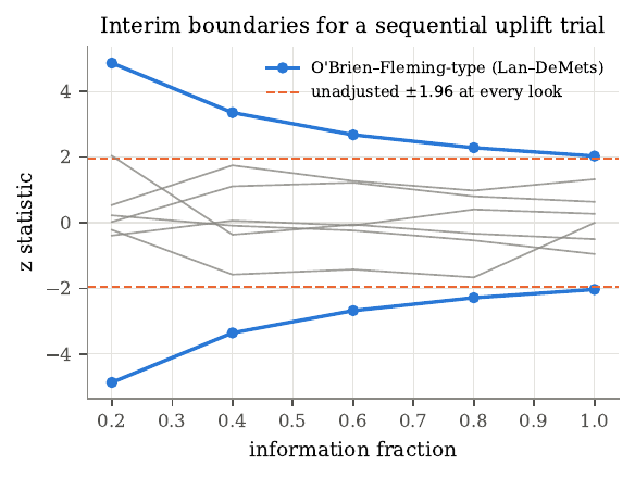
Figure 31. Group-sequential boundaries for an uplift trial with five equally spaced looks. Blue, O’Brien-Fleming-type boundaries from the Lan-DeMets spending function. Orange, the unadjusted \(\pm 1.96\) boundary. Grey lines are sample paths of the \(z\) statistic under the null hypothesis.

For five equally spaced looks at \(\alpha = 0.05\), the library returns \(z\) boundaries of 4.87, 3.36, 2.68, 2.29, and 2.03, which agree with published tables to within the grid resolution. Interim looks are safe only with boundaries fixed in advance.

Ethics and generalization

Uplift trials expose participants to model outputs and to tasks related to biological harm, so an institutional review board should review each trial, which should use proxy tasks safe to carry out and include monitoring and stopping rules. Three issues are specific. Information exposure, which calls for vetting recruits in proportion to task sensitivity, agreements not to retain materials, and storage at the appropriate tier; off-protocol actions, for which a one-sided exact binomial test can stop the trial if a monitored safety-event rate in the treatment arm exceeds a pre-specified maximum; and publication, where the aggregate effect size is usually safe to report but details of which tasks showed the largest effect may not be. A helpful-only treatment arm raises exposure substantially and belongs only with heightened vetting and an explicit review-board finding, with a transcript-review design as a lower-exposure alternative.

A well-run trial estimates uplift for its participants, on its proxy tasks, with its version of the model, while the decision concerns a different population, on actual tasks, with the deployed model and whatever follows. The largest external-validity gaps are that participants are vetted volunteers, that proxy tasks are graded on paper and omit physical difficulties, and that models change quickly. Statistics leave these gaps open, so you should treat the trial as one data point for calibrating capability evaluations, and that calibration holds only for the tasks, participants, and model versions the trial covered.

From scores to decisions

An evaluation ends in a decision. Clear a model under standard safeguards, flag it as requiring stronger ones, or judge the evidence insufficient and order more evaluation. Frontier developers’ safety policies define capability thresholds that trigger such decisions (Anthropic, 2023; OpenAI, 2023; Google DeepMind, 2024). The choice of who bears the burden of proof changes the outcome as much as the data do.

Burden of proof

Let the true capability score be \(\mu\) and the threshold \(\tau\), with \(k\) successes in \(n\) items. A rule-out rule clears the model only if the one-sided upper bound is below \(\tau\), so uncertainty counts against clearance and a model with too few items stays uncleared,

\[\text{clear} \iff U_{1-\alpha}(k, n) < \tau.\]

A rule-in rule flags the model only if the one-sided lower bound exceeds \(\tau\), so uncertainty counts against flagging,

\[\text{flag} \iff L_{1-\alpha}(k, n) > \tau.\]

The library uses exact Clopper-Pearson bounds for both, since a safety decision is a setting where guaranteed coverage is worth some conservatism. A rule-out rule is precautionary, placing the burden on showing safety, which matches most frontier safety policies. Anthropic gave a public example when it activated its AI Safety Level 3 protections for Claude Opus 4, stating that it had not determined the model crossed the relevant threshold but could not rule it out, and applied the stronger protections as a precaution (Anthropic, 2025). A rule-in rule places the burden on showing danger, the posture of a regulator who must justify a restriction. Each rule carries a posture, and a report should state which it uses.

Three-way decisions

Applying both rules partitions every result into cleared, flagged, or inconclusive, and inside the inconclusive band the right output is a call for more evaluation and no verdict.

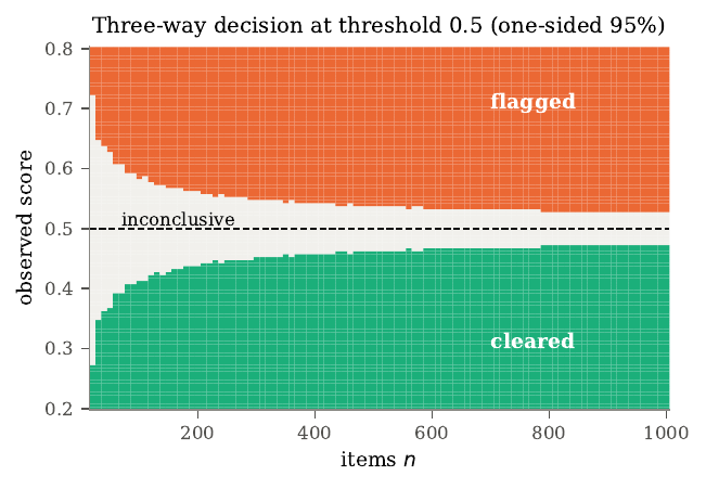
Figure 32. Three-way decision regions for a threshold of 0.5 with one-sided 95 percent Clopper-Pearson bounds. Green, cleared under the rule-out rule. Orange, flagged under the rule-in rule. Grey, inconclusive. The inconclusive band narrows as the number of items grows.

The band is wide when \(n\) is small and narrows at rate \(1/\sqrt{n}\). With 100 items any observed score between about 0.42 and 0.58 is inconclusive, and with 1,000 items the band narrows to about 0.47 to 0.53. A model whose true score is near the threshold needs many items to leave the band. For a threshold of 0.5, a model with true score 0.30 resolves with 30 items, one at 0.40 needs 80, one at 0.45 needs 285, and one at 0.48 needs 1,705, since the requirement grows as the inverse square of the distance to the threshold. This is a strong argument for targeted and adaptive testing, spending budgets on the models that sit near thresholds.

Bayesian exceedance and asymmetric loss

Frequentist bounds answer how surprising a result would be if the true score were at the threshold, but decision makers often want the probability that the true score exceeds the threshold given the data. With a Beta\((a, b)\) prior and \(k\) successes in \(n\) items, the posterior is Beta\((a + k, b + n - k)\) and the exceedance probability is

\[\Pr(\mu > \tau \mid k, n) = 1 - F_{\text{Beta}(a+k,\, b+n-k)}(\tau).\]

Letting \(L_{\text{clear}}\) be the cost of clearing a model above the threshold and \(L_{\text{flag}}\) the cost of flagging one below, flagging minimizes expected loss when the exceedance probability exceeds

\[p^* = \frac{L_{\text{flag}}}{L_{\text{flag}} + L_{\text{clear}}}.\]

If a decision maker judges clearing a dangerous model to be 20 times as costly as flagging a safe one, the critical probability is \(1/21 \approx 0.048\), so flag the model whenever it has roughly a 5 percent chance of exceeding the threshold. Writing down the cost ratio converts an implicit judgment into an explicit, arguable number. A uniform prior Beta\((1,1)\) is a common default, and a prior informed by the previous generation’s score is more realistic but, if too strong, can hide a sudden jump in capability, so reports should show results under a weak prior and any informed prior used.

Aggregating evidence, and policies as rules

A biosecurity assessment rarely rests on one evaluation, and two aggregation logics point in opposite directions. When several independent evaluations test the same construct, Fisher’s method combines their \(p\)-values through \(-2\sum_{i} \log p_{i}\), which follows a \(\chi^2\) distribution with \(2m\) degrees of freedom under the null; in practice different evaluations of one construct share items, graders, or elicitation, so they are rarely independent and Fisher’s method overstates the combined evidence, and pooling at the level of item responses through a joint IRT model is more faithful. When evaluations test different steps of a pathway the logic reverses, because the pathway succeeds only if every step succeeds, so clearing a model on the grounds that it fails one step requires a strong evaluation of that step, and a step with no evaluation counts as inconclusive by default. Absence of evidence about a step is not evidence that the step is hard.

Published frontier safety policies can be read as decision rules of this kind. Anthropic’s Responsible Scaling Policy defines AI Safety Levels with capability thresholds, including for chemical, biological, radiological, and nuclear weapons, and requires stronger safeguards once a model reaches a threshold or the developer cannot rule it out (Anthropic, 2023). OpenAI’s Preparedness Framework tracks risk categories including biological and chemical capability (OpenAI, 2023), and Google DeepMind’s Frontier Safety Framework defines critical capability levels with early-warning evaluations (Google DeepMind, 2024). Where a policy states a threshold in terms of uplift but tests it with capability evaluations, it relies on the proxy assumption, a policy judgment no measurement has tested. Policies usually leave the statistical form of the rule unspecified in public, such as which bound is compared with the threshold, at what confidence level, and how many items or participants it requires; making these choices explicit, even internally, would make decisions more consistent and easier to audit. For early-warning designs, the gap between the warning threshold \(\tau_{\text{warn}}\) and the critical threshold \(\tau\) should exceed the expected capability gain between evaluations plus the width of the inconclusive band, or a model can cross from below the warning level to above the critical level between rounds, with both rounds missing it.

To run all of it end to end, I build a benchmark, run two simulated models through the harness, compute intervals and a paired comparison, place both models on an IRT ability scale, apply a three-way decision rule, and produce tiered reports. Every number comes from the worked-example script’s output, and because the items are placeholders and the models are simulators, the true values are known.

I create 240 placeholder items in 4 constructs, grouped 4 to a scenario, and split by cluster into a 60-item development set, used to choose the prompt and elicitation, and a 180-item held-out set on which I compute every number. The blueprint check shows each construct has 45 items from 45 scenarios, and the power formula already says that construct-level scores from 45 items will have intervals roughly \(\pm 0.13\) wide, so construct-level differences of a few points carry no meaning. Knowing this before running the evaluation prevents over-reading the per-construct table later.

The harness sends each item to the model five times, shuffling option order on each sample, parses each response, detects refusals, and scores the parsed choice against the key after undoing the shuffle. The transcript sink writes PUBLIC transcripts to an ordinary file and higher-tier transcripts to a secure writer, keeping only a reference built from the item fingerprint, the sample index, and a hash of the text; in a verification run over 80 items with 4 samples each, the public file contained 124 lines, equal to the 31 PUBLIC items times 4 samples, and no restricted transcript reached it. Each run also writes a content-free manifest with a hash of all item fingerprints and a configuration digest, which lets an auditor confirm the item set and configuration.

I evaluate two models, both 3PL simulators with fixed abilities \(\theta_{A} = -0.2\) and \(\theta_{B} = 0.6\), in a helpful-only configuration so they answer every item and the score targets capability. A third run evaluates model B’s deployed configuration, which refuses 60 percent of samples on RESTRICTED items, scored with refusals as incorrect so it targets propensity. The scores and their uncertainty follow.

	model A	model B
true expected score	0.659	0.772
observed score	0.656	0.771
naive SE	0.0196	0.0189
clustered SE	0.0225	0.0192
design effect	1.31	1.03
effective items	137	174
95% CI (clustered)	[0.611, 0.700]	[0.734, 0.809]
95% CI (cluster bootstrap)	[0.612, 0.699]	[0.734, 0.809]
between-item variance	0.030	0.036
mean within-item variance	0.196	0.141
SE floor as \(K \to \infty\)	0.0129	0.0141

Both scores are within one standard error of the true expected scores. For model A clustering inflates the variance by about 31 percent and the effective sample size falls from 180 to 137, while for model B the design effect is 1.03; the difference is why each model needs its own design effect. The clustered normal and cluster bootstrap intervals agree to within 0.002. For model A the within-item variance is about 6.5 times the between-item variance, so about six or seven samples per item would be reasonable, and with five the standard error of 0.0196 is about 50 percent above the floor of 0.0129.

Because both models answered the same items, I pair the comparison with cluster-robust standard errors. Model B scores 0.116 higher than model A, with a paired clustered standard error of 0.0174 and a 95 percent interval of [0.081, 0.150]. An unpaired analysis would give a standard error about 56 percent larger because it ignores the positive correlation between the two models’ item outcomes. The true difference of 0.114 lies inside the interval, the minimum detectable difference for this benchmark is about 0.12, and a benchmark of this size would often miss a smaller true difference. The deployed configuration of model B refused 17.9 percent of all samples and, with refusals scored as incorrect, scored 0.646 against the capability score of 0.771, a different question about how often a user of the deployed system would receive a correct answer, where the capability score measures how much the model knows.

To place the models on a stable scale, I calibrate the item parameters on a panel of 40 other respondents with the 3PL model and guessing floors fixed at 0.25. The calibration converged, recovered difficulties with correlation 0.90, and produced no negative discriminations, so there is no sign of key errors. Model A has estimated ability \(-0.15\) (posterior SD 0.18) against a true \(-0.14\), and model B has \(0.66\) (SD 0.19) against a true \(0.55\), both within one posterior SD. With a threshold of \(\tau = 0.70\) and a rule-out burden of proof, applied to the effective sample size to respect clustering, model A’s one-sided 95 percent bounds are [0.585, 0.724]. The upper bound exceeds 0.70, which blocks clearance, and the lower bound sits below 0.70, which blocks flagging, so the outcome is inconclusive, and the posterior exceedance probability is 0.12 under a uniform prior. Model B’s bounds are [0.712, 0.822], so its lower bound exceeds the threshold and it is flagged, with posterior exceedance 0.98. Model A’s true score is about 4 points below the threshold, and with 137 effective items the evaluation leaves it uncleared, so the appropriate response is to add items targeted near the threshold, keeping the result as the data give it.

Finally the pipeline builds construct-level rows and renders a controlled view at full precision and a public view that coarsens scores and interval limits to the nearest 0.05 and suppresses any slice with fewer than 20 items or 5 clusters. The public construct-level intervals are about 0.15 to 0.20 wide, too wide to compare constructs within a model, and the evaluation card lists this limitation explicitly. The worked example demonstrates that the blueprint check predicted uninformative construct-level comparisons before any model ran, that clustering changed the effective sample size differently for the two models, that pairing reduced the comparison’s standard error by about a third, that the propensity and capability scores answer different questions, and that a model 4 points below the threshold stayed uncleared with 137 effective items.

Reporting comes last, and a biosecurity evaluation has several audiences. The team needs every detail, internal decision makers need the decision and its basis, external auditors need enough to check the reasoning, and the public needs to know what was tested and found at a level that does not spread hazardous information. One set of result records should serve all of them, so no audience sees a number the others lack and no hazardous content leaves the secure environment.

The pipeline stores each result as a record with the construct, model, score, interval, item and cluster counts, refusal rate, the maximum tier of the items behind the row, and the decision. The controlled view returns every field at full precision and goes, under agreement, to vetted evaluators and auditors. For the public view, two transformations apply. Coarsening rounds scores and interval limits to a grid, by default 0.05, which limits how much a set of published aggregates reveals about individual items, since an attacker who sees many full-precision slices can sometimes infer outcomes on small groups, and it also discourages over-interpretation of differences smaller than the measurement can support. Small-cell suppression removes any slice with fewer than a minimum number of items or clusters, by default 20 items and 5 clusters, borrowing from official statistics. These two rules are a starting point with no formal privacy guarantee; formal methods such as differential privacy would add a quantified leakage budget at the cost of extra noise.

An evaluation card applies the idea of model cards (Mitchell et al., 2019) and datasheets (Gebru et al., 2021) to an evaluation, documenting what it is for and how the team built and ran it while holding out all item content. The card records purpose and estimand, threat-model reference, constructs and blueprint, items by tier, validation, elicitation, grading and grader reliability, statistics and minimum detectable difference, contamination controls, and known limitations. The known-limitations field is the most important, because every biosecurity evaluation measures a proxy and every proxy has gaps, and a card that lists them lets readers calibrate their trust.

The guiding rule is to publish methods in full, results in aggregate, and content only at the public tier. Methods carry no information hazard, and publishing them lets others check and reuse the design. Publish results through the public view with coarsening, suppression, and labeled estimands. Publish item content, keys, rubrics, and transcripts only at the public tier, and choose any public subset from the lowest hazard tier and label it as unrepresentative of the full evaluation’s difficulty, since the most sensitive items are usually also the hardest. When an evaluation discovers something hazardous, such as a prompting strategy that bypasses a safeguard, I handle it with responsible-disclosure norms from computer security. Report it privately to the developer with enough detail to fix it, wait to describe it publicly until a fix is in place, and then describe it at a level of generality that informs other developers while withholding a recipe, with a suggested default of notifying the developer’s security contact before any preprint and holding a 90-day embargo. Restricted content limits who can check an evaluation, which controlled auditor access to the secure environment and a manifest of item fingerprints and a configuration digest together address (US AISI and UK AISI, 2024; Raji et al., 2020). A public summary can follow a fixed structure. Question and estimand, evaluation card, results, decision and burden of proof, limitations, and access.

The battery, as a checklist

The thread through all of it is that the failure stays hidden in the headline number and surfaces once you add the control. So I run the same battery on any score before I trust it, written here as a checklist. Five tests, each with the one measurement that exposes the failure it is built to catch, and each one appeared earlier in this guide either as a statistical derivation or as a case study.

Test 1, beat a trivial baseline

Before a score gets credit for understanding, it has to beat the simplest thing that could work. For a protein variant, that is the number of mutations it carries. Score your variants with the model and with a plain mutation count, within each study, and compare rank correlations to the measured outcome. The fail signal is the model scoring at or below the count, as on the PET-hydrolase variants above. Always compare inside the unit a campaign would act on, because pooling across assays lets between-study offsets look like signal.

Test 2, measure utility in the top tail

Benchmarks report a correlation over a whole assay. A campaign keeps the top few candidates. Those are different quantities, and the first stops predicting the second where you use it. For each benchmark unit, measure the value of the designs selected at a sharp cutoff and ask how much the reported correlation predicts that selection value. The fail signal is that the relationship decays as selection sharpens, the decay in Figure 2, and some assays with positive correlation give worse-than-random top-1 percent selections.

Test 3, control the obvious confound

If the plainest property of the input reproduces a movement in a representation, it gives no evidence about the mechanism you are studying. Build a control that preserves the confound, amino-acid composition or sequence length, and destroys the structure you are claiming, and measure how much of the effect survives. The fail signal is that most of it survives the control, as in the PRISM steering result earlier. Report the size of what is left, because the sign alone falls short.

There is a general reason confounds pass for mechanisms, and my meeting notes name it simplicity bias. Gradient descent prioritizes easily separable, low-frequency linear features, such as background color or texture, over complex nonlinear causal structure, going by those notes, which I have not verified. When a model latches onto a superficial feature that also correlates with the label, the score looks healthy and the model has still missed the causal structure. A confound control is how you find out which case you are in.

Test 4, hold whole groups out

Decodability on familiar examples is the evidence people cite most for understanding, and it is the easiest to overread. Train your probe or policy, then evaluate on entire groups, whole mechanisms or whole families, held out of training. Random splits fall short here. The fail signal is that performance collapses out of distribution, as the PRISM recommender does earlier. A random split would have hidden this completely.

My meeting notes give this failure a name, the behavioral alignment fallacy. Identical outward behavior can rest on radically different internal strategies, and standard metrics can report high alignment from superficial correlations, which my notes flag as a caution I still need to verify. A probe that scores well on familiar data is a behavioral match. The held-out-group test asks whether anything behind the behavior transfers. The same notes warn about a sharper version of the trap. If a brain and a network both latch onto the same superficial feature, RSA can score high while the model misses the deep causal structure. That is a false-positive alignment score, and it is why decodability on familiar examples leaves the question open.

Test 5, null against the selection

When a search keeps the top candidate, the right null mimics the selection at the same budget. The kept candidate has the largest error among many, so with $$s = f^{*} + \varepsilon$$ the quantity $$\mathbb{E}[\max_{i\le n}\varepsilon_{i}]$$ grows with $$n$$ and the selected error inflates the score on its own. Compare your selection to a null that mimics the selection procedure at the same budget, and report where the score and the realized quality first separate. The fail signal is that the apparent gain is selected error. This is also why a safety benchmark can be half-answered from the options alone, which is the WMDP-Bio case study earlier, and why reporting the best of several elicitation conditions biases a capability estimate upward.

What to report

For every score, publish the trivial baseline, the top-k utility next to the bulk correlation, the confound control with the size of the surviving effect, the held-out-group result, and the selection-matched null. If a verifier is in the loop, red-team it in a setting where ground truth exists, as above, where a leaked scorer cleared a trust gate and added nothing, so you had to measure detection and recovery separately. Two forward versions of this come next. A white-box evaluation asks whether an assay property is even recoverable from a model internal activations and whether that recovery survives a shift to unfamiliar families. A portable check wraps any score, runs bounded search against it, and reports where the score and the actual quality first separate, so the check travels across domains and stays general.

Back to the opening question. When a model aces a benchmark for biology, what you have learned is that it is good at the benchmark, and whether it is good at the task is a separate claim that needs the battery above. The practical version is short. Report top-k utility next to bulk correlation, publish the trivial baselines and the confound controls, hold whole groups out, and let a search attack the score before anyone keys a decision to it.

I want to be clear about the limits of this argument. Each result here is a demonstration on one codebase, model, or dataset, several reuse a small set of assays, and the protocol is a hypothesis about which diagnostics predict failure, short of a theorem. The direction has held every time I have looked. The most important models will move outside the distribution where their scores were calibrated, and the evidence we trust about them should be built for that setting from the start.

The methods in this guide are mature in the fields they come from, but their application to biosecurity evaluation leaves several problems open. The link between capability scores and uplift is the weakest link in current practice, since most organizations set capability thresholds by expert judgment because uplift data are scarce. A direct way forward is to embed short capability evaluations in every uplift trial, so each trial adds a data point relating capability to measured uplift, and to pool such data across organizations at the level of aggregate effect sizes using random-effects meta-analysis; the obstacle is coordination and trust, with statistics already in hand. Measuring tacit knowledge is a second gap, since many steps depend on hands-on skill that written evaluations may systematically misjudge, and multimodal items (Götting et al., 2025) and benign laboratory tasks with physical outcomes may be the only ways to measure the construct directly. Formal disclosure control for evaluation results is a third, since coarsening and suppression are heuristics while differential privacy offers formal guarantees whose trade-off against the already limited precision of these benchmarks is not yet understood.

Benchmarks saturate quickly while expert-validated items are slow and costly to write, so dynamic benchmarks (Kiela et al., 2021) adapted to this domain, with IRT linking items written at different times onto one ability scale, are a direction, as is using models to help draft items for expert review, which raises its own information-hazard questions. Current methods for detecting sandbagging are indirect and inconclusive, and as models become more evaluation-aware (Laine et al., 2024) the assumption that a model tries its best becomes harder to justify, so methods that inspect internal representations are a promising but immature direction. Specialized biological design tools raise different measurement problems (Sandbrink, 2023; Urbina et al., 2022), since their outputs are sequences or structures whose function only laboratory work can confirm and whose successful evaluation produces among the most hazardous artifacts in the field. Finally, clinical trials have reporting standards such as CONSORT (Schulz et al., 2010) and biosecurity evaluations have no equivalent; a short agreed list of required elements, covering the estimand, interval method, clustering adjustment, refusal policy, decision rule, and minimum detectable effect, would make results comparable across organizations at little cost, and I offer the evaluation card and section checklists as a starting draft.

Responsible use. This guide and its companion library cover measurement methodology only. They contain no pathogen names, no description of acquisition, enhancement, production, or dissemination, and no item content. Threat pathways appear only as abstract structures with unnamed steps, all items are placeholder strings, and all responses come from simulation. Before posting, I reviewed the manuscript and code against a non-uplift measurement standard covering admissible inputs, the absence of any optimisation or generation loop over biological content, and aggregate-only release. An external advisor reviewed the release and is the contact for questions about responsible use. Readers who build their own evaluations with these methods should keep item content, answer keys, rubrics, and transcripts under the access controls described above. The open problems on model-assisted item drafting and biological design tool evaluation involve hazardous inputs or outputs, and no one should pursue them without separate safety review.

As for provenance and thanks, PRISM was supervised independent research with AITHYRA, with Gabriela Lobińska, and I presented it as an oral at IEEE CIBCB 2026. The checking code is in the protein-lm-audits repository. biologos is independent research, a measurement in place of a bid to build a better model, with code at github.com/saanviiyer/biologos. I wrote up the measurement-and-statistics machinery and its companion library biosec_eval as a standalone guide, and every statistical number in it comes from a simulator with fixed seeds.

Supplementary derivations

Standard error of a chance-corrected score. The chance-corrected score is a linear function of the raw score, and for \(g(x) = (x - u)/v\) the variance scales by \(1/v^2\), so

\[\operatorname{SE}(\hat\mu_{\text{corr}}) = \frac{\operatorname{SE}(\hat\mu)}{1 - 1/k} = \frac{k}{k-1}\,\operatorname{SE}(\hat\mu).\]

For four-option items the corrected standard error is \(4/3\) times the raw one. Chance correction stretches the scale, and the uncertainty stretches with it.

The binomial-Beta identity behind Clopper-Pearson. The limits rest on

\[\Pr(X \ge k \mid n, p) = \Pr(B \le p), \qquad X \sim \text{Binomial}(n, p),\; B \sim \text{Beta}(k, n - k + 1).\]

Drawing \(n\) uniforms, the event that at least \(k\) fall below \(p\) is the event that the \(k\)-th smallest is at most \(p\), and the \(k\)-th order statistic of \(n\) uniforms is Beta\((k, n-k+1)\). The lower Clopper-Pearson limit is therefore the \(\alpha/2\) quantile of Beta\((k, n-k+1)\), and the upper limit follows symmetrically.

Consistency of the cluster-robust variance. Writing \(E_{c} = (T_{c} - m_{c}\mu) - m_{c}(\hat\mu - \mu)\), the first term has mean zero and variance \(\Var(T_{c})\), and the second is of order \(m_{c}/\sqrt{C}\), so summing squares over clusters gives \(\sum_{c} E_{c}^2 = \sum_{c} \Var(T_{c})(1 + O(1/C))\) in expectation and the estimator is consistent as the number of clusters grows. The factor \(C/(C-1)\) removes the leading downward bias. Consistency requires many clusters, and adding items within a cluster leaves it unchanged, which is why the estimator is unreliable with few scenarios.

Unbiased estimation of within-item variance. For an item with true probability \(p\) and \(K\) samples with mean \(\bar y\),

\[\mathbb{E}[\bar y(1 - \bar y)] = p(1-p)\,\frac{K-1}{K},\]

so multiplying by \(K/(K-1)\) gives an unbiased estimator of \(p(1-p)\), and averaging over items gives \(\sigma_{w}^2\). Since the sample variance of item means has expectation \(\sigma_{b}^2 + \sigma_{w}^2/K\), subtracting the estimated \(\sigma_{w}^2/K\) gives \(\sigma_{b}^2\), truncated at zero in small samples.

Unbiasedness of the pass@\(k\) estimator. Let \(S\) be a uniformly random \(k\)-subset of the \(n\) outcomes, chosen independently, and \(A = 1\) if \(\max_{i \in S} Y_{i} = 1\). Conditional on the outcomes, \(\Pr(A = 1) = 1 - \binom{n-c}{k}/\binom{n}{k}\), the estimator itself. Because \(S\) is independent of the i.i.d. outcomes, \(\{Y_{i} : i \in S\}\) is a set of \(k\) i.i.d. Bernoulli\((p)\) variables, so the expectation is \(1 - (1-p)^k\). The same argument with the minimum gives the pass\(^k\) estimator.

Delta-method variance of the Rogan-Gladen estimator. With \(g(o, s, t) = (o + t - 1)/(s + t - 1)\) and \(J = s + t - 1\), the partial derivatives are \(1/J\), \(-g/J\), and \((1-g)/J\), so for independent samples

\[\Var(\hat\pi) \approx \frac{1}{J^2}\left[\Var(\hat\pi_{\text{obs}}) + \pi^2\,\Var(\widehat{\mathrm{Se}}) + (1 - \pi)^2\,\Var(\widehat{\mathrm{Sp}})\right].\]

The factor \(1/J^2\) inflates all variance when the grader is weak, and the weight \((1-\pi)^2\) means that for low pass rates uncertainty in specificity dominates.

A numerical example of non-collapsibility. Split a population evenly into low-skill and high-skill participants, with skill balanced across arms, and suppose model access doubles the odds of success in both strata. Among low-skill participants success rises from 0.10 to about 0.182, and among high-skill from 0.50 to about 0.667, a conditional odds ratio of 2 in each stratum. Averaging, control success is 0.30 and treatment is 0.424, so the marginal odds ratio is

\[\frac{0.424/0.576}{0.30/0.70} \approx 1.72,\]

smaller than the conditional 2 despite no confounding. The marginal risk difference, \(0.424 - 0.30 = 0.124\), is often the most useful summary, and standardization recovers it from the adjusted model (Kahan et al., 2014).

Fisher information of a Bernoulli outcome. For \(\ell(\theta) = y\log p + (1-y)\log(1-p)\), the score is \(\ell'(\theta) = p'(y - p)/[p(1-p)]\), and since \(\mathbb{E}[(y-p)^2] = p(1-p)\),

\[I(\theta) = \frac{(p')^2}{p(1-p)}.\]

Beyond those derivations, I run every estimator in the companion library on data simulated from a known generative model, with all seeds fixed, to confirm that the code implements the formulas in the text and that each formula recovers what it claims in the setting described. The checks and their results follow.

• Interval coverage (400 benchmarks of 200 items in scenarios of 8, nominal 95 percent): naive 90.8 percent; clustered 94.8 percent.
• Design effect (one benchmark from the same generator): deff 1.20; estimated \(\rho\) 0.028.
• IRT recovery (60 respondents, 300 items, 2PL joint MAP): correlation 0.99 for ability, 0.94 for difficulty, 0.62 for discrimination; converged.
• Targeted subset (new respondent at \(\theta = 1.0\), 30 items): targeted \(0.89 \pm 0.25\); random \(1.13 \pm 0.44\); all 300 items \(0.97 \pm 0.14\).
• pass@\(k\) (\(p = 0.15\), \(n = 20\), \(k = 5\), 20,000 replicates): estimate 0.558; truth 0.556.
• Time horizon (60 tasks, 1 to 960 min, 8 runs; true \(h_{50} = 45\), \(\beta = 0.9\)): estimated \(h_{50} = 53.6\) minutes [43.1, 66.0]; \(\beta = 0.94\).
• Uplift power (\(p_{0} = 0.10\), \(p_{1} = 0.25\), planned 80 percent power, 1,000 trials): \(n = 100\) per arm; empirical power 82.1 percent.
• Covariate adjustment (120 per arm, \(p_{0} = 0.2\), conditional odds ratio 2, 1,000 trials): power unadjusted 50.9 percent; adjusted 58.4 percent.
• O’Brien-Fleming bounds (5 equally spaced looks, two-sided \(\alpha = 0.05\)): 4.870, 3.358, 2.680, 2.287, 2.034 (tables: 4.877, 3.357, 2.680, 2.290, 2.031).
• Continuous sample size (80 percent power, \(\alpha = 0.05\)): \(d = 0.2\) needs 393; \(d = 0.5\) needs 63; \(d = 0.8\) needs 25 per arm.
• Minimum detectable effect (50 per arm, \(p_{0} = 0.10\)): 0.220.
• Rogan-Gladen (true rate 0.12, Se 0.85, Sp 0.95, gold set 100 positives and 200 negatives): observed 0.146; corrected 0.120 [0.063, 0.170].
• Items to resolve (threshold 0.5, one-sided 95 percent exact bounds): true 0.30 needs 30; 0.40 needs 80; 0.45 needs 285; 0.48 needs 1,705.
• Harness routing (80 items, 4 samples, 31 PUBLIC items): 124 public lines.
• Refusal policy (40 percent random refusal on RESTRICTED items, true expected score 0.718): missing 0.733; incorrect 0.644.
• Winner’s curse (100 items, equal true scores 0.5): best of 2 adds 2.8 points; of 4, 5.1; of 8, 7.1; of 16, 8.8.
• Items needed (paired, \(p = 0.5\), no pairing benefit, 80 percent power): \(\delta = 0.10\) needs 393; 0.05 needs 1,570; 0.02 needs 9,812.

Two results deserve comment. The time-horizon estimate of 53.6 minutes is 19 percent above the true 45, but the bootstrap interval contains the truth and the overestimate is consistent with sampling error at 60 tasks. The covariate-adjustment gain is smaller than the continuous-outcome variance-reduction formula would suggest, because for binary outcomes with logistic regression part of the apparent gain comes from the change of estimand, and the simulation reports actual power in place of the approximation.

Key references

• Anthropic (2023). Anthropic’s Responsible Scaling Policy.
• Anthropic (2025). Activating AI Safety Level 3 Protections.
• Birnbaum, A. (1968). Some latent trait models and their use in inferring an examinee’s ability.
• Brown, L. D., Cai, T. T., and DasGupta, A. (2001). Interval estimation for a binomial proportion.
• Chen, M., Tworek, J., Jun, H., et al. (2021). Evaluating Large Language Models Trained on Code.
• Clopper, C. J., and Pearson, E. S. (1934). The use of confidence or fiducial limits illustrated in the case of the binomial.
• Cohen, J. (1960). A coefficient of agreement for nominal scales.
• Google DeepMind (2024). Frontier Safety Framework.
• Götting, J., Medeiros, P., Sanders, J. G., et al. (2025). Virology Capabilities Test (VCT): A Multimodal Virology Q&A Benchmark.
• Kwa, T., West, B., Becker, J., et al. (2025). Measuring AI Ability to Complete Long Tasks.
• Laurent, J. M., Janizek, J. D., Ruzo, M., et al. (2024). LAB-Bench: Measuring Capabilities of Language Models for Biology Research.
• Li, N., Pan, A., Gopal, A., et al. (2024). The WMDP Benchmark: Measuring and Reducing Malicious Use with Unlearning.
• Lord, F. M. (1980). Applications of Item Response Theory to Practical Testing Problems.
• Messick, S. (1995). Validity of psychological assessment.
• Miller, E. (2024). Adding Error Bars to Evals: A Statistical Approach to Language Model Evaluations.
• Mouton, C. A., Lucas, C., and Guest, E. (2024). The Operational Risks of AI in Large-Scale Biological Attacks: Results of a Red-Team Study.
• Newcombe, R. G. (1998). Interval estimation for the difference between independent proportions.
• OpenAI (2023). Preparedness Framework (Beta).
• O’Brien, P. C., and Fleming, T. R. (1979). A multiple testing procedure for clinical trials.
• Patwardhan, T., Liu, K., Markov, T., et al. (2024). Building an Early Warning System for LLM-Aided Biological Threat Creation.
• Phuong, M., Aitchison, M., Catt, E., et al. (2024). Evaluating Frontier Models for Dangerous Capabilities.
• Rogan, W. J., and Gladen, B. (1978). Estimating prevalence from the results of a screening test.
• Sandbrink, J. B. (2023). Artificial Intelligence and Biological Misuse: Differentiating Risks of Language Models and Biological Design Tools.
• Schulz, K. F., Altman, D. G., and Moher, D. (2010). CONSORT 2010 Statement.
• Shevlane, T., Farquhar, S., Garfinkel, B., et al. (2023). Model Evaluation for Extreme Risks.
• Wilson, E. B. (1927). Probable inference, the law of succession, and statistical inference.