Apical Dust: Brain-inspired Backprop-Free Pretraining

TL;DR. The brain learns continually from a forward process, which raises two questions I tested. First, whether a biologically plausible, local learning rule retains more than backpropagation. Second, whether borrowing more of the brain’s machinery trains a network well in place of backpropagation. On class-incremental Split-CIFAR-10 with a fair comparison, local rules forget at about the backpropagation rate. Once I match each rule to backpropagation at the same learning accuracy, locality’s retention margin is 0.21 points, and a plain replay buffer adds 10.6. Rehearsal accounts for the gain. For the second question, I added a learned top-down feedback pathway, modeled on cortical apical dendrites, to Q Labs’ Dust, the first zeroth-order method that pretrains transformers about as well as backpropagation. As an unbiased control variate it is worth about 1.6 to 2 times the population at small draw counts, at about the same wall-clock cost, and the gain fades by 256 draws. Two methodological findings matter beyond the biology. Per-step cosine to backpropagation ranks gradient estimators backwards when their bias differs, and Dust’s token embeddings need credit from future tokens. Backpropagation stays ahead at this scale.

The brain learns from local signals

My background is in neuroscience, and the starting point for all of this is a plain fact from systems neuroscience. The cortex learns forward. Backpropagation needs two things a biological circuit lacks. It needs the backward path to use the exact transpose of the forward weights, the weight-transport problem, and it needs a global error signal threaded precisely backward through every layer. Biological synapses update from local quantities. Roughly presynaptic activity, postsynaptic activity, and a neuromodulatory third factor that stands in for reward or surprise. That is three-factor plasticity, and it is local in both space and time.

There is a fourth ingredient the brain uses that machine learning rarely copies. Top-down feedback arrives on a separate part of a cortical pyramidal neuron, the apical dendrite, and tells the cell which way to change. I will come back to it in the second half.

Researchers usually frame this gap between brains and backpropagation as a problem for biological plausibility. It is just as interesting as a question about machine learning, and it splits into two questions. If the brain learns continually, across a lifetime, from a forward process and from a small sample of past experience, then whatever it is doing is a candidate solution to catastrophic forgetting, the failure where a network trained on a new task overwrites the weights that encoded the old one. And if a backprop-free rule can be pushed to train as well as backpropagation, then the brain’s extra machinery might be the thing that pushes it there. The first half of this post tests the forgetting question and finds the answer small. The second half takes up the training question and finds a smaller effect that holds up.

The appealing version of the forgetting question is that locality itself buys retention. A backpropagation update couples every weight to every other through the global error, so learning a new task can move any weight that mattered for an old one. A local rule moves a weight only from signals available at that synapse, so the intuition goes, it should disturb unrelated structure less and forget less. Feedback alignment, direct feedback alignment, and predictive coding are the usual bio-plausible candidates, and some reports credit all three with forgetting less than backpropagation.

The trouble with that literature is a confound that is easy to miss. A rule that learns each new task less well also has less to forget. If a method only reaches 70% on the new task where backpropagation reaches 90%, it has written less into the shared weights, so of course it overwrites less of the old task. Read on its own, its better retention is partly just weaker learning. Comparing forgetting across methods is valid only once you hold learning fixed. I was suspicious going in, because in most of the papers I read the local rule arrived bundled with something else, like sparsity or replay, and the write-ups credited the retention to locality anyway.

Each of these three rules assigns credit in a different way, sidestepping backpropagation’s weight transport.

• Feedback alignment keeps the forward pass and sends the error backward through fixed random weights in place of the transpose of the forward weights, so the network learns from fixed random connections alone.
• Direct feedback alignment goes further and sends the output error straight to each hidden layer through its own fixed random connection, skipping the layer-by-layer backward chain.
• Predictive coding has each layer try to predict the activity of the layer below it, and the local mismatch between prediction and actual activity drives learning, which under some conditions approximates backpropagation using only local signals.

All three are biologically motivated, and reports credit all three with helping on forgetting. The rest of this half asks whether that help holds up once the comparison is fair.

A fair test that separates forgetting from learning

The first thing to build is a measuring instrument. I weakened backpropagation across eleven settings that vary only the number of epochs and the learning rate, holding out any mechanism that protects old tasks, and measured backward transfer, the change in accuracy on earlier tasks after training on later ones, as a function of how well the network learned the new task. The task is class-incremental Split-CIFAR-10, five tasks of two classes each with a single growing head and no task labels at test time, which is the hard version of the problem, and I ran Split-CIFAR-100 and Split-FashionMNIST as replications. Every arm trains the same two-layer network, so the learning rule is the only thing that changes.

Within each seed, backward transfer turned out to be almost a deterministic function of learning accuracy, with an \(R^2\) of 0.995. Holding out each setting in turn, that relationship predicts backward transfer to a mean absolute error of 1.09 points over 224 held-out predictions, which tells me how small a difference I can trust. That tight relationship is the instrument. With it in hand I scored each rule against backpropagation at the same learning accuracy, tuned the baseline as hard as the rule, and corrected each remaining difference for the small accuracy gap left over.

pause apparent edge of locality +4.3 pts

Matched this way, the bio-plausible rules stop looking special. Under matched learning accuracy, feedback alignment differed from backpropagation by -0.08 points, with a 95% interval of [-0.21, +0.05], and direct feedback alignment by -0.11, [-0.28, +0.06]. Both intervals contain zero, so both rules forget at about the backpropagation rate once the baseline is tuned fairly. Predictive coding retained 0.21 points more, [+0.11, +0.31], p = 0.001. I had said ahead of time that a local rule retaining better at matched learning would refute my hypothesis, so I report predictive coding as a refutation, and I note that 0.21 points is about a fifth of the instrument’s own error and that the gap correction alone flips its sign. I read this as the locality advantage being an artifact of a baseline that was allowed to learn more. Locality of credit assignment, the property people reach for, leaves forgetting about where it was.

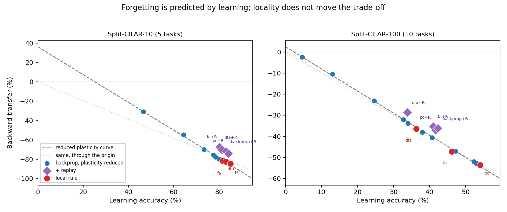
Figure 1. Backward transfer against learning accuracy on Split-CIFAR-10 and Split-CIFAR-100. The backpropagation ladder traces the trade-off between learning a new task and forgetting earlier ones, so local rules that fall on the curve forget about as much as backpropagation at a matched learning accuracy, and only replay sits above it. Locality moves you along the trade-off. It does not shift the trade-off itself.

What reduces forgetting is old and simple. Replay, which I added as a positive control, rehearses a small sample of earlier data while learning the new task, and it improved retention by 10.6 points, [+10.0, +11.1], about fifty times the predictive-coding effect. Rehearsal accounts for the gain. This matches a plain reading of the brain too. The hippocampus replays experience during rest and sleep, and replay is among the most clearly established biological mechanisms for retention.

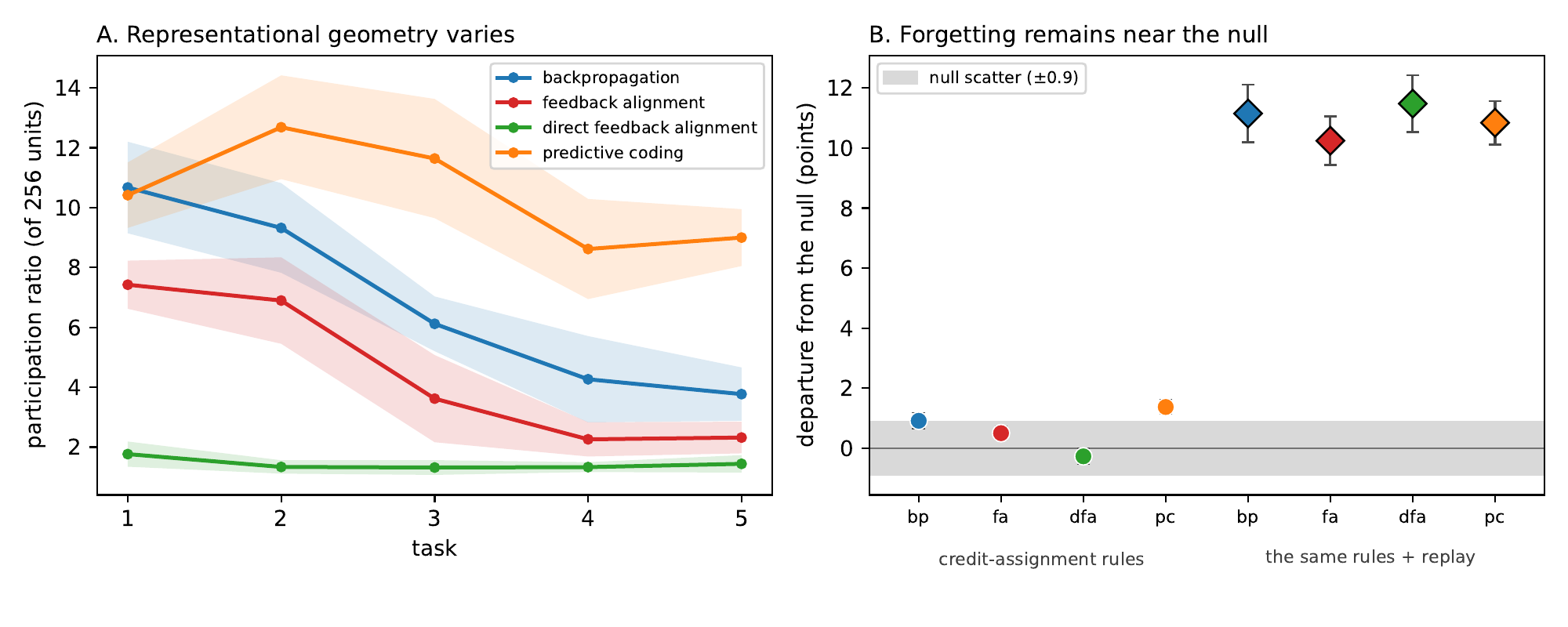
Figure 2. Departure from the null for each learning rule, with and without replay. Each credit-assignment rule sits inside the null band, the scatter expected from rules that do nothing special for retention, while adding replay lifts every arm about ten points above it. The left panel shows the representational geometry differs between rules, but that difference does not become a difference in forgetting.

One limit belongs right next to that number. Split-CIFAR-10 with a growing head keeps little to begin with, about 0.7 points, so the setup sits near a floor where little forgetting remains to prevent. When I rescored within each task’s own classes to lift it off that floor the ordering held, with replay still ahead and the local rules matched, though the instrument then resolved retention only to about five points. Split-FashionMNIST was too noisy to serve as a quantitative instrument, at 12.29 points of held-out error, so I withhold retention differences from it. The defensible scope is Split-CIFAR-10 and Split-CIFAR-100 under this protocol.

The conclusion from the continual-learning side is a null, and it is worth stating cleanly because the opposite is so often assumed. A learning rule being local, or brain-like in its credit assignment, leaves catastrophic forgetting about where it was. This matters past neuroscience. When a deployed model keeps training, through fine-tuning or reinforcement learning from human feedback, it can erase abilities and safety behaviors it had before, which is catastrophic forgetting with a deployment address. If your method claims to protect earlier behavior, the first question to ask is whether the comparison held learning of the new task fixed against backpropagation.

A more constructive question

A null result on one framing is an invitation to change the framing. The new question is whether adding a piece of cortical machinery to a backprop-free learner makes it train better in the first place. That is where Q Labs’ Dust comes in. Dust is the first zeroth-order method competitive with backpropagation at pretraining transformers, and it is a biologically flavored rule. Noise in the activations, a reward signal, and a local update, the same three ingredients as three-factor plasticity, running entirely on the forward pass.

There is a second reason to take backprop-free rules seriously, and it comes from the limits of backpropagation itself. In my meeting notes, backpropagation needs continuous differentiable operations, which excludes discrete jumps, open loops, and external program execution. Q-Labs describes backpropagation as an efficiency crutch that imposes rigid constraints on scaled compute, and proposes forward-pass search-based learning, with an analogy to AlphaGo Zero. That framing comes from Q-Labs.

Dust works by node perturbation, as described in my meeting notes. It injects Gaussian noise directly into the outputs of every linear layer per token. Older evolutionary strategies such as AGReL perturb weights, and weight perturbation suffers extreme variance across billions of parameters. Credit comes from Centered Loss Reduction, which subtracts the baseline mean loss of the perturbed variations, with a discount factor gamma for delayed multi-token credit.

The benchmark numbers in my meeting notes set the scale of what Dust does and where it stalls, and I give them in full in the next section. On the NOISE speedrun Dust matches backpropagation closely under SGD, then stalls once Adam and a learning-rate cooldown enter. The proposed mechanism in my notes is that per-step cosine similarity checks mask a systematic estimator bias. Memoryless SGD averages out zero-mean noise, while Adam’s momentum accumulates directional bias across steps and drives optimization off course.

I added one more cortical ingredient. Top-down feedback onto apical dendrites. Each layer gets a learned linear prediction of its own output error from the network’s output error, estimated from forward passes only, so the method stays entirely on the forward pass. In my meeting notes this mirrors pyramidal neurons, which receive top-down contextual feedback through apical dendrites as approximate learned signals. I fit the learned feedback map by ridge regression against true output errors and use it as an unbiased control variate, which subtracts a predictive baseline from token perturbations to suppress variance while keeping the estimate unbiased. The control variate matters most at small populations, 16 draws per token in my notes, and becomes redundant at 256 draws, where raw noise averages out on its own.

The rest of the post is that follow-up in detail. It is independent research, unaffiliated with Q Labs.

Dust looked familiar the moment I read it. It injects Gaussian noise into every layer’s output, scores each token’s noise by how much it lowered the loss, and forms the weight gradient from the reward-weighted noise. That is three-factor plasticity. Presynaptic activity, postsynaptic activity, and a neuromodulatory reward. The appeal for machine learning is concrete. A single forward pass tests thousands of perturbations at once, free of a backward pass and of weight transport, which is why it is competitive at pretraining where other zeroth-order methods stall. The deeper reason to look past the backward pass, in my notes, is that backpropagation needs continuous differentiable operations and so excludes discrete jumps, open loops, or external program execution.

Their follow-up, the Noise speedrun, argues that another 1,000-fold gain will need credit assignment, optimizers and architectures designed together. This post is a small, independent contribution to the credit-assignment and optimizer parts of that program.

Dust adds Gaussian noise to the output of every linear layer, independently at every token. In my meeting notes, this is node perturbation, which differs from older methods like AGReL that perturb weights and suffer extreme variance across billions of parameters. It rewards each token’s noise by how much that noise lowered the loss. Each token thus acts as one member of a population, and one forward pass tests thousands of perturbations. The reward-weighted noise estimates the error at each layer’s output. The outer product of that error with the layer’s input gives the weight gradient, which is the same update backprop forms.

In my meeting notes, Dust assigns credit through Centered Loss Reduction, which subtracts the baseline mean loss of perturbed variations, with a discount factor γ for delayed multi-token credit.

The cost is variance. With K draws and a d-dimensional layer output, the noise in the per-token estimate scales roughly with d/K. Dust reduces that noise by increasing the population, which costs compute. I wanted to know whether a biological mechanism could remove some of the noise more cheaply.

The Noise speedrun gives context for why small populations matter. In my meeting notes, the speedrun evaluates a 37.7M-parameter GPT model on 10M tokens from FineWeb, with zero backward passes allowed. Dust reached a record validation loss of 4.167 in 1.76 hours on 8 H100 GPUs. With SGD, the gap to backprop was 0.051. With Adam plus a learning rate cooldown, backprop improved to 3.769 while Dust stalled, widening the gap to 0.398. The proposed mechanism in those notes is that per-step cosine similarity masks bias. Memoryless SGD averages out zero-mean noise, while Adam momentum accumulates directional bias across steps. That mechanism matches the bias pattern I found at small scale, which is one reason I focus on the averaging test below. I treat the Q Labs view of backpropagation that frames all of this as their framing, something still short of established fact.

Feedback onto the apical dendrite

Cortical pyramidal neurons receive bottom-up input on their basal dendrites. Top-down feedback from higher areas arrives on a separate apical dendrite. Several models of cortical learning treat the apical signal as a local, approximate error that tells each neuron which way to change (Guerguiev, Lillicrap and Richards, 2017). The signal stays approximate, so the brain must learn it somehow. Lansdell, Prakash and Kording (2020) proposed that the brain learns its feedback weights from noise. Neurons jitter, a neuromodulatory reward reports the outcome, and the correlation between the two trains the feedback pathway. Dust already has the noise and the reward. It lacks the pathway.

Apical adds it. For every module \(m\), I keep a feedback matrix \(B_m\). It maps the network’s output error at a token, \(e_t\), to a predicted error at the module’s output.

\[\begin{aligned} \hat g_{\text{pred}}(t) &= B_m\, e_t \\ e_t &= \text{Dust estimate of } \partial \mathcal{L} / \partial\, \text{logits}_t \quad \text{(jitter the cached logits; no derivatives)} \\ B_m &= \text{EMA ridge regression of Dust's estimates } \hat g(t) \text{ on } e_t \end{aligned}\]

Every step stays zeroth-order. I estimate the output error by perturbing the logits, which costs only one more cross-entropy evaluation. I fit the feedback weights by regressing Dust’s noisy estimates on \(e_t\). The noise in those estimates is independent of \(e_t\), so it averages out of the fit.

In my meeting notes, I state the same idea in biological terms. Pyramidal neurons get top-down feedback through apical dendrites, carrying approximate learned signals in place of exact gradients. A learned linear feedback map, fit by ridge regression against true output errors, serves as an unbiased control variate. It subtracts a predictive baseline, and it suppresses variance while leaving the estimate unbiased.

A prediction of the gradient can enter the update in three ways. The ways differ in how much they trust the prediction.

1. Feedback only. Update with \(B_m e_t\) alone, as in learned feedback alignment (Lillicrap et al., 2016; Nøkland, 2016). Noise trains the pathway, and the prediction alone moves the weights. The variance is low, and the update is biased wherever a linear map from the output error falls short of the true gradient.

2. Control variate (Apical). Remove the part of each reward that the feedback already explains, estimate only the remainder from noise, and add the prediction back.

   \[\begin{aligned} r'(t) &= r(t) + \sigma \, \big\langle \hat g_{\text{pred}}(t),\, a(t) \big\rangle \\ \hat g(t) &= \hat g_{\text{pred}}(t) - \frac{1}{K\sigma} \sum_{k=1}^{K} r'_k(t)\, a_k(t) \end{aligned}\]

   In expectation, the correction term cancels the prediction, so the estimate stays unbiased for any \(B_m\). A poor feedback map therefore leaves the expected update unharmed. Its noise now scales with the size of the remainder \(g - \hat g_{\text{pred}}\) in place of \(g\).

3. Precision-weighted. Shrink the remainder toward the prediction according to its estimated reliability. Predictive-coding models of cortex weigh prediction errors by precision in this way (Feldman and Friston, 2010). I estimate the reliability online from how well the two halves of the population agree.

Setup

Every run fits on a laptop GPU.

• Data: character-level tiny Shakespeare (65 symbols), split 90/5/5 into train, validation and test.
• Model: GPT-style transformer with 2 layers, width 128, 4 heads and context 64. Each step uses 8 sequences (512 tokens), for 1000 steps.
• Optimizer: SGD with momentum 0.9 and a constant learning rate. I tuned the rate per method and population on seed 0, over {0.003, 0.01, 0.03, 0.1} at K=16 and 64, and over {0.01, 0.03} at K=256. Each cell then runs three seeds at the tuned rate. A seed fixes the initialization and the data order, so I can pair seeds across methods.
• Metric: test loss at the best validation checkpoint, as in the Dust paper.
• Populations: K = 16, 64 and 256. K counts draws per module per step. Each of the 13 jittered modules gets its own K draws, and the logits get 4K.

My Dust is a faithful but simplified reimplementation. It uses one noise scale (σ = 0.05) for every layer, and its layer norms use a fixed gain. In the first version, I credited attention keys and values with a discounted sum of future token losses (γ = 0.9). The paper scores them by alignment with the error at the attention output. Result 4 replaces my rule with the paper’s. Absolute numbers will differ from the paper’s numbers.

First I measured the per-step cosine between each estimate and the backprop gradient on the same batch, at a partly trained checkpoint. The Dust paper uses the same alignment analysis. By this measure the feedback is a clear win. At K=16, the precision-weighted estimate on the MLP input layer reaches 0.78, which is higher than Dust reaches at K=256. Feedback alone does almost as well on most layers. The unbiased control variate falls between the two. Going in, I read Figure 3 as strong support for the feedback, and Result 2 is where that reading broke.

● Dust   ● Apical (unbiased)   ● Precision-weighted   ● Feedback only

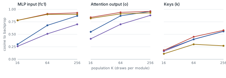
Figure 3. Per-step alignment with backprop. Cosine between each estimated weight gradient and the backprop gradient on the same batch, against population, averaged over layers of each type and 4 batches. Checkpoint is 300 backprop steps. Feedback fitted for 40 steps before measuring.

Training disagreed with Figure 3. The estimate with the best per-step cosine trained the worst. At K=16, the precision-weighted version trained worse than plain Dust, even with about three times the per-step cosine. Per-step cosine mixes two kinds of error. Noise is fresh every step, and momentum averages it out over roughly ten steps. Bias points the same way every step, so momentum adds it up.

To separate the two kinds of error, I fixed one batch and averaged more and more independent K=16 estimates. The cosine of an unbiased estimator approaches 1 as the average grows. A biased estimator levels off below 1, at a height set by its bias. Dust and the control variate keep rising, and on the values layer both reach 0.92 at 256 estimates. The feedback-based estimates stall. On the keys layer they barely move, 0.14 for feedback only and 0.37 for precision-weighted, against 0.91 for Dust.

The keys show the cause. Later tokens read the key at token t, so the true gradient of that key depends on errors that occur after t. The feedback pathway sees only the error at t, so it misses that credit. The same limit applies, less severely, to values, and to any gradient that depends on a token’s own Jacobian, which a single linear map averages away.

● Dust   ● Apical (unbiased)   ● Precision-weighted   ● Feedback only

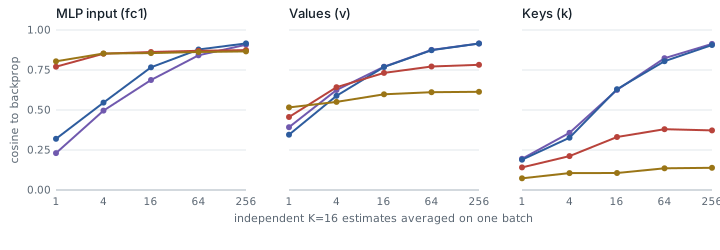
Figure 4. Averaging separates noise from bias. Cosine to the backprop gradient of the mean of N independent K=16 estimates on a single fixed batch. Unbiased estimators (Dust, Apical) keep rising toward 1. Biased ones (feedback only, precision-weighted) level off. The embedding layers (not shown) level off near 0.7 for every method. Result 4 traces that plateau to Dust’s credit rule for embeddings.

This result bears on tuning Dust. The Dust paper shortlists noise scales and credit decays by their cosine to backprop on a single batch, then lets training choose among them. A single-batch cosine rewards any change that trades noise for bias. The averaging curve costs a few hundred extra estimates on one batch, and it shows the bias as the height where the curve levels off. I would use that height as the screen.

In my meeting notes, the corresponding action item is a bias check that measures cosine similarity of Dust estimates against true gradients across sample sizes from 1 to 4,096, to confirm persistent bias plateaus. That is the same test, run wider.

The statistic that ranks estimators backwards

Here is the finding I would put in front of the Dust team, because it changes a decision they make in practice. I think it is the most useful thing I found here. The Dust paper shortlists hyperparameters by measuring the cosine similarity between an estimator’s update and the true backpropagation gradient on a single batch. That statistic ranked my estimators backwards.

A feedback-weighted estimator triples per-step cosine on the MLP, from 0.26 to 0.78 at \(K=16\), and still trains worse, by 0.044 nats. The reason is that its error points the same way every step, and momentum sums that bias up over training. A single-batch cosine misses this, because on any one step the biased estimator does point close to the gradient. What separates bias from noise is averaging. Average each estimator’s updates over many batches and compare the average to backpropagation. Noise averages out and reveals the unbiased estimator. A biased estimator’s average stays stuck at an angle however many batches you add.

pause averaged cosine to backprop, feedback-weighted 0.00, control variate 0.00

If single-batch cosine is the filter that picks which estimator or hyperparameter to scale, it will prefer the biased one, which looks aligned every step and quietly accumulates error through momentum. The averaging test costs one extra loop and gives the right ordering. Recall that the control-variate estimator contrasted here is the feedback map fit by ridge regression against true output errors.

The same bias story shows up in my meeting notes at NOISE scale, in the speedrun numbers above. My notes describe the same variance pattern at larger scale as well, with the control variate mattering most at 16 draws per token and becoming redundant at 256 draws, where raw noise averages out on its own. I report those meeting-notes numbers as what they are, and they need checking before anyone leans on them.

Kept unbiased, the feedback helps where Dust is noisiest. Apical has lower test loss than Dust in every seed-paired comparison at K=16 and K=64. It also varies less across seeds, which is what variance reduction should do. I had expected that from a control variate, and watching the seed spread shrink made me trust the mechanism more. At K=256 the advantage is gone. Apical wins 2 of 3 pairs, by -0.001 on average.

Method	K = 16	K = 64	K = 256
Dust	2.510 ± 0.006	2.488 ± 0.010	2.473 ± 0.001
Apical (unbiased control variate)	2.498 ± 0.004	2.478 ± 0.004	2.473 ± 0.001
Apical − Dust, paired	-0.012 (3 of 3)	-0.010 (3 of 3)	-0.001 (2 of 3)
Precision-weighted	2.554 ± 0.004	2.487 ± 0.007	not run
Feedback only	2.634 (1 seed)	not run	not run
Backprop	2.394 ± 0.007

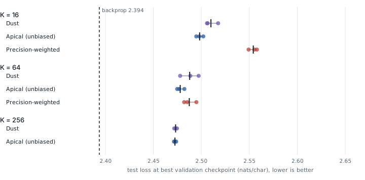
Figure 5. Final test loss across the population ladder. Dots are seeds, the black tick is the mean, and the dashed line is backprop. Feedback only is left out because it was run on one seed.

▬ Backprop   ● Dust   ● Apical (unbiased)   ● Precision-weighted

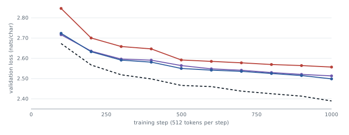
Figure 6. Validation loss during training at K=16, mean of 3 seeds. The precision-weighted version falls behind within the first hundred steps and never catches up.

To express the K=16 gain as population, I interpolated Dust’s loss log-linearly between K=16 and K=64. Apical at K=16 matches Dust with about 33 draws, roughly twice the population. Apical closes about 53% of the gap between Dust at K=16 and Dust at K=64.

In my meeting notes, the control variate substantially reduces variance at small virtual population sizes, for example 16 draws per token, and becomes redundant at large population sizes, for example 256 draws, where raw noise averages out naturally. That matches what I measured.

Equal population can still mean unequal cost, so I timed both methods. In the sweep, my first Apical implementation took about twice as long per run as Dust at K=16. At that price, Dust could double its population and match Apical. Almost all of the overhead was waste. The code repeated a clean forward pass and a logit jitter, computed split-half estimates even when they went unused, and inverted a 65-by-65 matrix that forced a GPU-to-CPU sync every step. The method itself adds one small matrix product per module plus the regression update. That is about 1% of the arithmetic of the perturbed forward passes.

With the waste removed, the median step time of Apical relative to Dust, over three interleaved rounds, was 0.86x at K=16, 1.22x at K=64 and 0.95x at K=256. Other jobs shared the machine, so I read these times as equal within about 20%. The optimized code does the same math with a different random stream. One K=16 run with it reached 2.500, against 2.502 for the original code on the same seed. At K=16 the gain is worth about a doubling of population, which is well above a 20% cost, so the gain survives matched compute. My first implementation would have erased it.

The averaging test also locates the remaining bias in Dust itself. I ran the same averaging test on Dust’s own estimates to see where its bias still sat. With 1024 independent estimates averaged on one batch, my original Dust reaches cosine 0.98 on queries, attention outputs and the MLP. It reaches only 0.88 on keys and values and 0.71 on the token embedding. Two credit rules explain the gap. First, my reimplementation credited keys and values with a discounted sum of downstream token losses, which is cruder than the paper’s rule. Second, it credited each embedding only for its own token’s loss. The Dust paper makes the same choice. As I read its Section 2.3, only keys, values, gates and value embeddings receive credit from future tokens. However, the embedding at token t enters the residual stream, and later tokens read it through attention, so its true gradient includes their losses.

I made two changes. For attention internals I implemented the paper’s rule. It jitters queries, keys or values, recomputes only that block’s attention output from cached activations, and scores each jitter per head by its alignment with the estimated error at the attention output. Keys and values also get credit from later tokens (γ = 0.97). For embeddings, where the paper stops short of this, I added future-token credit (γ = 0.9). In the averaging test, keys rise from 0.88 to 0.95 and the token embedding from 0.71 to 0.78, still climbing at 1024 estimates. Values stay near 0.87, so some bias remains there.

My meeting notes add one adjacent credit-assignment detail. Dust applies a discount factor gamma for delayed multi-token credit, with gamma equal to 0.9 in the action plan recorded there. That is the same family of problem as the embedding fix. Credit has to reach the place and time where it belongs, and the places it misses show up as a stall.

Both changes make each single estimate noisier, so training has to decide. The embedding credit carries most of the gain. The attention rule alone hurts at K=16, where its extra noise costs more than the bias it removes. Combined with the embedding credit, it helps at larger populations.

Test loss, nats/char	K = 16	K = 64	K = 256
Original Dust (my reimplementation)	2.510 ± 0.006	2.488 ± 0.010	2.473 ± 0.001
+ paper’s attention credit	2.529 ± 0.005	2.484 ± 0.006	not run
+ future credit for embeddings	2.502 ± 0.006	2.464 ± 0.003	2.446 ± 0.006
+ both (fixed Dust)	2.509 ± 0.001	2.452 ± 0.016	2.443 ± 0.006
Fixed − original, paired	-0.001 (1 of 3)	-0.036 (3 of 3)	-0.030 (3 of 3)
Apical on fixed Dust	2.489 ± 0.004	2.444 ± 0.014	not run
Apical − fixed Dust, paired	-0.020 (3 of 3)	-0.008 (1 of 3)	not run
Backprop	2.394 ± 0.007

I tuned learning rates on seed 0 over {0.01, 0.03} at K=16 and 64. At K=256 the fixed variants reuse 0.03 directly. That rate won for them at K=64 and for the original Dust at K=256.

The row closest to the paper’s Dust is “+ paper’s attention credit”. Adding embedding credit to it lowers mean test loss from 2.529 to 2.509 at K=16 and from 2.484 to 2.452 at K=64. These are differences of means, pooled across seeds. Against my original Dust, the fixed version lowers test loss by 0.036 at K=64 and 0.030 at K=256, which closes about 38% of the K=256 gap to backprop. The fixed Dust at K=64 already beats the original at K=256. Its ladder still flattens, gaining only 0.009 from K=64 to K=256, so bias still sets the floor.

On the fixed Dust, the feedback pathway gains more at K=16, -0.020 in all three seed pairs, against -0.012 on the original. The averaging test predicts this. The fixed estimator is less biased but noisier per step, and noise is what a control variate removes. In population terms, the gain equals about 1.6 times the population on the fixed Dust’s steeper ladder. At K=64 the difference is -0.008, with one of three pairs better, which is inconclusive. Apical on the fixed Dust at K=16 reaches 2.489, level with the original Dust at K=64 (2.488) with a quarter of the draws.

What I would test at Dust’s scale

My runs cover the low end of Dust’s population ladder on a toy task. The Dust paper runs from K=64 to 16k on FineWeb with models up to 243M parameters. A few checks would show whether these mechanisms carry over.

The first check is the embedding credit, which costs nothing to try. With a context of 64 tokens and 2 layers, the embedding stalled at 0.71. With longer contexts and more layers, more later tokens read each embedding, so I expect the truncation bias to grow. The averaging test on one FineWeb batch would show this in minutes.

The second is the averaging plateau as a tuning screen. If the paper’s cosine-picked candidates differ from the plateau-picked ones, the training runs will show which screen is right.

The third is the control variate across the full ladder. A control variate removes variance, so its gain should shrink as K grows, as it did here. Its value is at small populations, and a compute-bound speedrun lives at small populations. A richer feedback map is the natural extension. Because the control variate keeps the estimate unbiased, a nonlinear map, or one that also sees future errors for keys and values, keeps the expected update at least as good. It can only predict more of the gradient or less.

In my meeting notes, the remaining action items are to tune the sequence-level token discount, with γ = 0.9, to deploy the learned apical feedback map into Noise training scripts to stabilize small-batch variance, and to re-evaluate post-bias-correction performance across both SGD and Adam to confirm closure of the 0.398 loss gap. My notes close with a matching set of checks. Measure cosine similarity of Dust estimates against true gradients across sample sizes from 1 to 4,096 to confirm whether a persistent bias plateau is there, tune the discount, and re-evaluate post-correction performance across both SGD and Adam to confirm whether the 0.398 gap closes. All of it comes down to measuring Dust with a statistic that can tell bias from noise.

Limitations

The continual-learning result is scoped to class-incremental Split-CIFAR-10 with a growing head, which sits near a retention floor, and the architectures compared are feedforward convolutional networks, so this speaks to credit-assignment rules under this protocol. Its scope stops at feedforward rules, and a wider-window replication on recurrent or sequential ones is the obvious next step.

The apical result is a demonstration on a specific backprop-free rule at small model scale. One small model, one character-level dataset, 512k training tokens and SGD only. Dust’s effects appear at much larger scale, and mine may fade there. Three seeds per cell. The improvement at K=16 and 64 is consistent (6 of 6 pairs) but small, between -0.001 and -0.020 per pair. Populations of 16, 64 and 256 only, and Apical on the fixed Dust at 256 remains unrun. I chose the credit decays (γ = 0.97 for keys and values, 0.9 for embeddings) from gradient cosines on one batch, ahead of any training. Timings come from a shared laptop GPU and are accurate to about 20%, the trained results use the first implementation, and I checked the optimized one on one seed only. The feedback map is linear in the current token’s output error. Backprop is still ahead at this scale. It reaches 2.394 nats against 2.443 for the best Dust at K=256.

Both experiments stop short of a claim about the brain itself. They are claims about what specific brain-inspired mechanisms do inside specific networks, measured against a baseline tuned as hard as the method.

Acknowledgements

The continual-learning work grew out of the NeuroAI track of the Neuromatch program, where I spent the summer on brain-inspired learning algorithms. It is otherwise independent research, and I will release the code when the project is public. The Dust follow-up is independent research, unaffiliated with Q Labs.

References

1. Dahal, Mandal, Gülbahar and Vegesna. Dust: Pretraining Transformers Without Backpropagation. Q Labs, 2026. qlabs.sh/research/dust
2. Lansdell, Prakash and Kording. Learning to solve the credit assignment problem. ICLR, 2020.
3. Guerguiev, Lillicrap and Richards. Towards deep learning with segregated dendrites. eLife, 2017.
4. Lillicrap, Cownden, Tweed and Akerman. Random synaptic feedback weights support error backpropagation for deep learning. Nature Communications, 2016.
5. Nøkland. Direct feedback alignment provides learning in deep neural networks. NeurIPS, 2016.
6. Frémaux and Gerstner. Neuromodulated spike-timing-dependent plasticity, and theory of three-factor learning rules. Frontiers in Neural Circuits, 2016.
7. Fiete and Seung. Gradient learning in spiking neural networks by dynamic perturbation of conductances. Physical Review Letters, 2006.
8. Feldman and Friston. Attention, uncertainty, and free-energy. Frontiers in Human Neuroscience, 2010.
9. Werfel, Xie and Seung. Learning curves for stochastic gradient descent in linear feedforward networks. NeurIPS, 2003.